Building a Predictive Typing Model
Everyone using a smartphone or a mobile device has used an onscreen smart keyboard that tries to predict the next set of words that the user might want to type. Typically, upto 3 words are predicted, which are displayed in a row at the top of the keyboard. Given that typing on a glass pane without tactile feedback, could be very frustrating at times, the smart keyboard goes a long way in alleviating these issues.
But, how does predictive typing work? Basically, it’s a predictive typing model built using an ngram with backoff prediction model. Makes complete sense, right? Well, it’s less complicated than it sounds, and actually not hard to understand, as we shall see further.
Corpus
To begin, we need a large corpus of text with a wide-ranging vocabulary. The first name that comes to mind is that of William Shakespeare. Shakespeare wrote a number of plays and poems that are classics in the English language. These plays and poems are available in the public domain and are easily accessible through a number of sources, (see here and here). By some accounts, Shakespeare’s vocabulary ranged from 15,000-30,000 words, which makes it excellent to use it for our corpus.
David Robinson’s gutenbergr package makes it easy to download ‘The Complete Works Of Shakespeare’, from Project Gutenberg’s website. The downloaded dataset is a data frame with text appearing in rows along with the gutenberg id.
dfRaw <- gutenberg_download(100)
knitr::kable(head(dfRaw, 12))| gutenberg_id | text |
|---|---|
| 100 | Shakespeare |
| 100 | |
| 100 | This Etext has certain copyright implications you should read! |
| 100 | |
| 100 | <<THIS ELECTRONIC VERSION OF THE COMPLETE WORKS OF WILLIAM |
| 100 | SHAKESPEARE IS COPYRIGHT 1990-1993 BY WORLD LIBRARY, INC., AND IS |
| 100 | PROVIDED BY PROJECT GUTENBERG ETEXT OF ILLINOIS BENEDICTINE COLLEGE |
| 100 | WITH PERMISSION. ELECTRONIC AND MACHINE READABLE COPIES MAY BE |
| 100 | DISTRIBUTED SO LONG AS SUCH COPIES (1) ARE FOR YOUR OR OTHERS |
| 100 | PERSONAL USE ONLY, AND (2) ARE NOT DISTRIBUTED OR USED |
| 100 | COMMERCIALLY. PROHIBITED COMMERCIAL DISTRIBUTION INCLUDES BY ANY |
| 100 | SERVICE THAT CHARGES FOR DOWNLOAD TIME OR FOR MEMBERSHIP.>> |
knitr::kable(dfRaw[sample(nrow(dfRaw), 6),])| gutenberg_id | text |
|---|---|
| 100 | Assure yourselves, will never be unkind. |
| 100 | |
| 100 | Like one besotted on your sweet delights. |
| 100 | And spurn in pieces posts of adamant; |
| 100 | Whereto, when they shall know what men are rich, |
| 100 | TITUS. Marcus, even thou hast struck upon my crest, |
Data Preparation
The copyright notice appears multiple times throughout the text. Fortunately, it doesn’t prevent us from using this data for non-commercial purposes. The first step is to merge the entire text and remove the copyright notices that are helpfully within << … >>. Secondly, in plays, the characters and their relationships and titles are defined with ‘DRAMATIS PERSONAE’. These lines have to be removed too.
After doing some quick cleaning, the text is reconverted to a data frame.
complete_works <- str_c(dfRaw$text, collapse = ".")
complete_works <- str_split(complete_works, "<<[^>]*>>")[[1]]
complete_works <- complete_works[!(str_detect(complete_works, "Dramatis Personae|DRAMATIS PERSONAE"))]
complete_works <- str_replace_all(complete_works, "\\[|\\]", ".")

dfContent <- as_tibble(complete_works) %>% slice(3:n())
rm(complete_works)
Finally, we parse the content into sentences. The tidytext package by David Robinson and Julia Silge, is most useful in doing this within the tidyverse framework.
Here’s what the function does below:
- Replaces all ‘logical’ sentence break delimiters by a period for easier tokenization by sentence
- Removes extra periods and spaces
- Tokenizes into sentences
- Removes all sentences containing ACT or SCENE
- Removes all digits from sentences
- Finally adds line numbers to each row (more on the importance of this later…)
A sample of 10 sentences is shown below.
getSentences <- function(dfContent) {
    df <- dfContent %>%
        mutate(value = str_replace_all(value, ";|:|!|\\?| \\-|\\- | \\- ", "\\. ")) %>%
        mutate(value = str_replace_all(value, "[\\.]+", "\\.")) %>%
        mutate(value = str_replace_all(value, "[[:space:]]+", " ")) %>%
        unnest_tokens(sentence, value, token = "sentences", to_lower = FALSE) %>%
        dplyr::filter(!str_detect(sentence, "Act|ACT|Scene|SCENE")) %>%
        mutate(sentence = str_replace_all(sentence, "[0-9]","")) %>%
        mutate(lineNumber = row_number()) %>%
        select(lineNumber, everything())
}

dfSentences <- getSentences(dfContent)
knitr::kable(dfSentences[sample(nrow(dfSentences), 10),])| lineNumber | sentence |
|---|---|
| 55991 | That with the King here resteth in his tent. . |
| 16097 | You are a merry man, sir. fare you well. |
| 9717 | He did ask favour. |
| 100749 | To the health of our general. . |
| 40908 | You are, I think, assur’d I love you not. |
| 117828 | Laurence. and another Watchman. |
| 19243 | Ere now denied the asker, and now again,. |
| 145024 | I swear to do this, though a present death. |
| 70942 | Stocking his messenger. |
| 122957 | For bringing wood in slowly. |
Creating ngrams
“ngrams are a contiguous sequence of n items from a given sequence of text…” - Wikipedia
In this case, ngrams would be a contiguous sequence of n words. In the simplest form, an ngram of size 1 is a single word. An ngram of size 2 or more is a set of words that appear one after the other in a sequence.
For instance, given a sentence - how are you doing?
- There are 4 Unigrams: how, are, you, doing
- There are 3 Bigrams: how are, are you, you doing
- There are 2 Trigrams: how are you, are you doing
- There is 1 Quadrigram: how are you doing
So, using the data frame of clean sentences that we parsed, the next step is to create ngrams.
Once again this is made simple using the unnest_tokens function from the tidytext package. And this is where grouping by line numbers is important because we want ngrams to be created by sequence of words, only within the same line. We do not want ngrams connected by a sentence break.
getNgrams <- function(dfSentences, n) {
    dfNgrams <- dfSentences %>%
        group_by(lineNumber) %>%
        unnest_tokens(word, sentence, token = "ngrams", n = n) %>%
        ungroup() %>%
        count(word, sort = TRUE) %>%
        rename(freq = n)
}
All Words
df1grams <- getNgrams(dfSentences, 1)
dim(df1grams)
[1] 26453 2
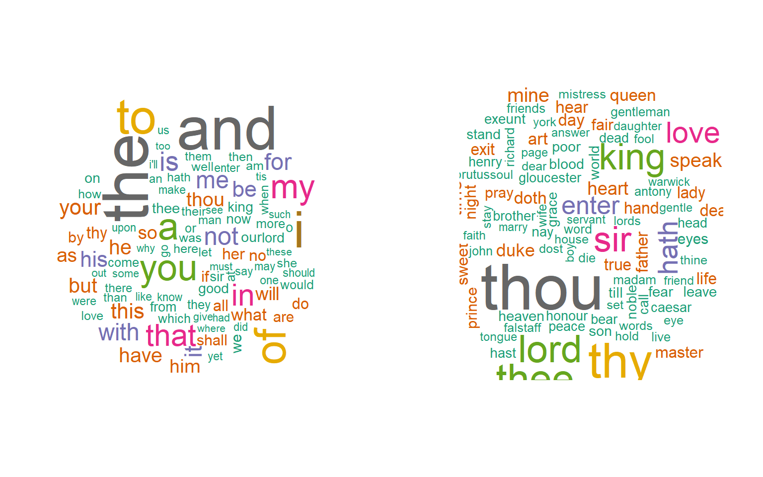
wordsOfFreq1 <- df1grams %>% group_by(freq) %>% summarise(n = sum(freq)) %>% dplyr::filter(freq == 1) %>% .$nThere are 26453 words in the corpus, that shows how vast Shakespeare’s vocabulary was. Let’s see a wordcloud of top 100 words. No surprise, the most commonly used words are: the, and, i, to, of. Excluding these commonly used ‘stop words’, in the second wordcloud, we can see the words Shakespeare used most frequently. We can see a lot of references to royalty and nobility, present specially in Shakespearean tragedies. Some names are mentioned quite frequently - Richard, John, Caesar, Brutus and Henry. Some English counties or shires are mentioned quite often - Warwick, York and Gloucester.
Unigrams
Let’s see a plot of the distribution of words in corpus by usage.
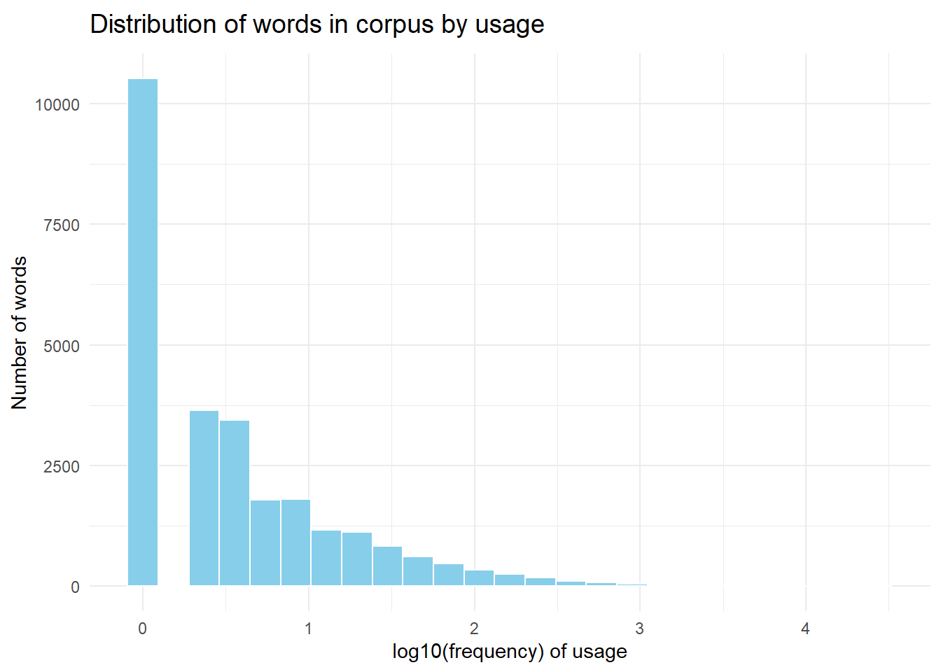
Here’s a strategy for building ngram tables:
- There is a long tail of 10522 words in the corpus that appear exactly once. Replace all words appearing just once, by UNK as a placeholder for a word not known from the corpus. There are a couple of motivations behind this:
- It reduces the size of ngram tables.
- More importantly, when an unknown word is encountered, the model knows how to tackle it before predicting the next set of words.
- Re-summarise and rearrange the table by frequency.
- Assign an index to each word.
- Convert to data.table format. Some of the biggest benefits of this approach are:
- Rows could be assigned and referenced by a key. This makes it extremely simple to look up a row value.
- Lookup by a key is very fast compared to matching character strings.
- When we create tables for bigrams and higher order ngrams, we can replace the words by their corresponding integer indexes. It saves a lot of memory as compared to creating tibbles with character strings.
vTopUnigrams <- df1grams %>% dplyr::filter(freq >= 2) %>% .$word
df1grams <- df1grams %>%
    mutate(word = ifelse(word %in% vTopUnigrams, word, "UNK")) %>%
    group_by(word) %>%
    summarise(freq = sum(freq)) %>%
    arrange(desc(freq)) %>%
    mutate(index1 = row_number()) %>%
    select(index1, freq, word)

dt1grams <- as.data.table(df1grams)
# set key to word
dt1grams <- dt1grams[,.(index1,freq),key=word]
# create another table with key=index1
dt1gramsByIndex <- dt1grams[,.(word,freq),key=index1]
# print dimensions
dim(dt1grams)
[1] 15932     3
Here are the top 10 unigrams. UNK replaces the long tail of words appearing once. Finally, we are left with 15932 unigrams in our table.
| index1 | word | freq | |
|---|---|---|---|
| 1 | 1 | the | 26821 |
| 2 | 2 | and | 25670 |
| 3 | 3 | i | 20473 |
| 4 | 4 | to | 19377 |
| 5 | 5 | of | 16954 |
| 6 | 6 | a | 14351 |
| 7 | 7 | you | 13568 |
| 8 | 8 | my | 12449 |
| 9 | 9 | in | 10881 |
| 10 | 10 | that | 10869 |
Bigrams
A data table of bigrams is created where the index of the first word is the lookup key. The second word cannot be UNK since it is a word used for making predictions from the bigram table.
df2grams <- getNgrams(dfSentences, 2) %>%
    separate(word, c("word1", "word2"), sep = " ") %>%
    mutate(word1 = ifelse(word1 %in% vTopUnigrams, word1, "UNK")) %>%
    dplyr::filter(word2 %in% vTopUnigrams) %>%
    group_by(word1, word2) %>%
    summarise(freq = sum(freq)) %>%
    arrange(desc(freq))

dt2grams <- as.data.table(df2grams)
dt2grams$index1 <- dt1grams[dt2grams$word1]$index1
dt2grams$index2 <- dt1grams[dt2grams$word2]$index1
dt2grams <- dt2grams[,.(index1,index2,freq)]
setkey(dt2grams, index1)

# print dimensions
dim(dt2grams)
[1] 254884      3
Here are the top 10 bigrams:
| word1 | word2 | freq | |
|---|---|---|---|
| 1 | 30512 | ||
| 2 | i | am | 1846 |
| 3 | my | lord | 1640 |
| 4 | in | the | 1611 |
| 5 | i | have | 1603 |
| 6 | i | will | 1553 |
| 7 | of | the | 1417 |
| 8 | to | the | 1380 |
| 9 | it | is | 1066 |
| 10 | to | be | 973 |
Trigrams
Similarly, a data table of trigrams is created where indexes of the first and second words form the lookup key. The third word cannot be UNK since it is a word used for making predictions from the trigram table.
df3grams <- getNgrams(dfSentences, 3) %>%
    separate(word, c("word1", "word2", "word3"), sep = " ") %>%
    mutate(word1 = ifelse(word1 %in% vTopUnigrams, word1, "UNK")) %>%
    mutate(word2 = ifelse(word2 %in% vTopUnigrams, word2, "UNK")) %>%
    dplyr::filter(word3 %in% vTopUnigrams) %>%
    group_by(word1, word2, word3) %>%
    summarise(freq = sum(freq)) %>%
    arrange(desc(freq))

dt3grams <- as.data.table(df3grams)
dt3grams$index1 <- dt1grams[dt3grams$word1]$index1
dt3grams$index2 <- dt1grams[dt3grams$word2]$index1
dt3grams$index3 <- dt1grams[dt3grams$word3]$index1
dt3grams <- dt3grams[,.(index1,index2,index3,freq)]
setkey(dt3grams, index1,index2)

# print dimensions
dim(dt3grams)
[1] 476098      4
From the top 10 trigrams, we can get an idea how UNK will be useful in this context. the UNK of is one of the most frequently used word sequences in the trigram table, which implies that if we encounter an unknown word after ‘the’, then ‘of’ is the most likely word to be predicted from the trigram table.
| word1 | word2 | word3 | freq | |
|---|---|---|---|---|
| 1 | 38526 | |||
| 2 | i | pray | you | 238 |
| 3 | i | will | not | 213 |
| 4 | i | know | not | 159 |
| 5 | i | do | not | 157 |
| 6 | the | UNK | of | 155 |
| 7 | the | duke | of | 141 |
| 8 | i | am | not | 139 |
| 9 | i | am | a | 138 |
| 10 | i | would | not | 127 |
Quadrigrams
Here are the top 10 quadrigrams:
| word1 | word2 | word3 | word4 | freq | |
|---|---|---|---|---|---|
| 1 | 47569 | ||||
| 2 | with | all | my | heart | 46 |
| 3 | i | know | not | what | 38 |
| 4 | give | me | your | hand | 31 |
| 5 | i | do | beseech | you | 31 |
| 6 | give | me | thy | hand | 30 |
| 7 | the | duke | of | york | 29 |
| 8 | i | do | not | know | 28 |
| 9 | i | would | not | have | 27 |
| 10 | ay | my | good | lord | 25 |
Pentagrams
Here are the top 10 pentagrams:
| word1 | word2 | word3 | word4 | word5 | freq | |
|---|---|---|---|---|---|---|
| 1 | 60534 | |||||
| 2 | i | am | glad | to | see | 15 |
| 3 | i | thank | you | for | your | 12 |
| 4 | i | had | rather | be | a | 9 |
| 5 | am | glad | to | see | you | 8 |
| 6 | as | i | am | a | gentleman | 8 |
| 7 | for | mine | own | part | i | 8 |
| 8 | i | pray | you | tell | me | 8 |
| 9 | know | not | what | to | say | 8 |
| 10 | and | so | i | take | my | 7 |
These ngram tables comprise all the information needed for the prediction model.
Memory Usage Comparison
As mentioned above, storing words as integer indexes in a data table is far more efficient as compared to a data frame with character strings. For instance, here’s how a pentagram data table looks like that contains just the integer indexes of the words:
| index1 | index2 | index3 | index4 | index5 | freq | |
|---|---|---|---|---|---|---|
| 1 | 1 | 1 | 1 | 9049 | 5 | 1 |
| 2 | 1 | 1 | 9049 | 5 | 1 | 1 |
| 3 | 1 | 4 | 2 | 9384 | 12918 | 1 |
| 4 | 1 | 4 | 687 | 31 | 4758 | 1 |
| 5 | 1 | 5 | 31 | 6421 | 29 | 1 |
| 6 | 1 | 9 | 183 | 2 | 1 | 1 |
| 7 | 1 | 11 | 1 | 46 | 15 | 1 |
| 8 | 1 | 11 | 1 | 57 | 16 | 1 |
| 9 | 1 | 11 | 1 | 1267 | 11402 | 1 |
| 10 | 1 | 11 | 1 | 1403 | 10842 | 1 |
In a comparison of memory needed for all ngram tables, we see a difference of a factor of 5 between the two approaches.
print(object.size(df1grams)+object.size(df2grams)+object.size(df3grams)+
          object.size(df4grams)+object.size(df5grams), units = "auto")
158 Mb

print(object.size(dt1grams)+object.size(dt1gramsByIndex)+object.size(dt2grams)+object.size(dt3grams)+
          object.size(dt4grams)+object.size(dt5grams), units = "auto")
30.4 Mb
Ngram With Backoff Prediction Algorithm
So, given the ngram data tables, here’s how the prediction algorithm works:
- Sanitize the input text as done above
- Parse the text into sentences
- Determine the words in the last sentence of the input text. Use upto the last 4 words from the input text.
- The word predictions are done starting from the ngram table containing the longest sequence of words, provided the input text contains atleast n-1 words. So, if the last 4 words from the input text match the first 4 words in the pentagram table, then the fifth word is chosen, that has the highest frequency of occurance after those 4 words. If more than one word prediction is desired, then the fifth words with the next highest frequency of occurance are also chosen.
- If no matches or fewer than desired number of matches are found in the pentagram table, then the algorithm backoffs to the quadrigram table using the last 3 words typed, then to the trigram table using the last 2 words typed, then to the bigram table using the last word typed and finally to the unigram table, until the desired number of word predictions are returned.
Let’s see how this works concretely with some test cases:
Test Cases
The first test is to confirm whether the word predictions from the unigram table, match with what we expect.
The top 10 unigram table contains 3 words beginning with the letter ‘t’ - the(1), to(4), that(10). And sure enough, this is what we get from our prediction function.
predictNextWords("t")
[1] "Predictions from 1grams: the,to,that,this,thou"
[1] "Top 3 Final Predictions: the,to,that"
From the bigram table, we could see that i am, i have and i will are among the top 10. So, the next test is to confirm these.
predictNextWords("i ")
[1] "Predictions from 2grams: am,have,will,do,would"
[1] "Top 3 Final Predictions: am,have,will"
Narrowing down to words that begin with letter ‘h’ gives us:
predictNextWords("i h")
[1] "Predictions from 2grams: have,had,hope,hear,heard"
[1] "Top 3 Final Predictions: have,had,hope"
Let’s predict some trigrams. i am not and i am a are among the top 10 trigrams, so that’s what we expect to see.
predictNextWords("i am ")
[1] "Predictions from 3grams: not,a,sure,glad,the"
[1] "Top 3 Final Predictions: not,a,sure"
Now let’s examine the UNK feature. We know that the UNK of is number 5 most common sequence in the trigram table so we should expect to see ‘of’ as the first prediction if the input text has an unknown word after ‘the’. So let’s input some gibberish after ‘the’ to make sure this word doesn’t exist in our vocabulary:
predictNextWords("the sjdhsbhbfh ")
[1] "Predictions from 3grams: of,and,in,that,the"
[1] "Top 3 Final Predictions: of,and,in"
Now that the known test cases are working well, let’s see the backoff algorithm in action:
predictNextWords("to be or not ")
[1] "Predictions from 5grams: to"
[1] "Predictions from 4grams: to"
[1] "Predictions from 3grams: to,at,i,allow'd,arriv'd"
[1] "Top 3 Final Predictions: to,at,i"
predictNextWords("to be or not to ")
[1] "Predictions from 5grams: be"
[1] "Predictions from 4grams: be,crack"
[1] "Predictions from 3grams: be,crack,the,have,me,do"
[1] "Top 3 Final Predictions: be,crack,the"
predictNextWords("be or not to ")
[1] "Predictions from 5grams: be"
[1] "Predictions from 4grams: be,crack"
[1] "Predictions from 3grams: be,crack,the,have,me,do"
[1] "Top 3 Final Predictions: be,crack,the"
predictNextWords("to be or not to be ")
[1] "Predictions from 5grams: that"
[1] "Predictions from 4grams: that,found,gone,endur'd,endured,seen"
[1] "Top 3 Final Predictions: that,found,gone"
predictNextWords("to be or not to be, that ")
[1] "Predictions from 5grams: is"
[1] "Predictions from 4grams: is,which"
[1] "Predictions from 3grams: is,which,you,he,i,thou,can"
[1] "Top 3 Final Predictions: is,which,you"
predictNextWords("to be or not to be, that is ")
[1] "Predictions from 5grams: the"
[1] "Predictions from 4grams: the"
[1] "Predictions from 3grams: the,not,my,to,a"
[1] "Top 3 Final Predictions: the,not,my"
predictNextWords("to be or not to be, that is the ")
[1] "Predictions from 5grams: question"
[1] "Predictions from 4grams: question,very,way,humour,best,brief"
[1] "Top 3 Final Predictions: question,very,way"
predictNextWords("be that is the ")
[1] "Predictions from 5grams: question"
[1] "Predictions from 4grams: question,very,way,humour,best,brief"
[1] "Top 3 Final Predictions: question,very,way"
Using one of the most well known speeches from Hamlet, we can see that the algorithm gets the first word prediction from the pentagram table. But since we are looking for the next 3 words, the algorithm backoffs to predictions from quadrigram and trigram tables, until it has atleast 3 words. In this case, the pentagram table gives us the best match that we are looking for. We can also observe that once we have atleast 4 words in our input text, the words prior to those do not matter for the next word predictions.
Let’s see another example:
predictNextWords("What a lovely day ")
[1] "Predictions from 5grams: "
[1] "Predictions from 4grams: "
[1] "Predictions from 3grams: "
[1] "Predictions from 2grams: and,to,is,of,i"
[1] "Top 3 Final Predictions: and,to,is"
predictNextWords("a lovely day ")
[1] "Predictions from 4grams: "
[1] "Predictions from 3grams: "
[1] "Predictions from 2grams: and,to,is,of,i"
[1] "Top 3 Final Predictions: and,to,is"
predictNextWords("lovely day ")
[1] "Predictions from 3grams: "
[1] "Predictions from 2grams: and,to,is,of,i"
[1] "Top 3 Final Predictions: and,to,is"
predictNextWords("day ")
[1] "Predictions from 2grams: and,to,is,of,i"
[1] "Top 3 Final Predictions: and,to,is"
Here we see that even though there are enough words to start matching from the higher ngram tables, the matches are gotten only from the bigram table using ‘day’ as the first word.
Another one:
predictNextWords("Beware the ides of ")
[1] "Predictions from 5grams: march"
[1] "Predictions from 4grams: march"
[1] "Predictions from 3grams: march"
[1] "Predictions from 2grams: march,the,my,his,a,this"
[1] "Top 3 Final Predictions: march,the,my"
predictNextWords("Beware the ides of mar")
[1] "Predictions from 5grams: march"
[1] "Predictions from 4grams: march"
[1] "Predictions from 3grams: march"
[1] "Predictions from 2grams: march,marriage,marcius,marcus,mars"
[1] "Top 3 Final Predictions: march,marriage,marcius"
predictNextWords("Beware the ides of march")
[1] "Predictions from 5grams: march"
[1] "Predictions from 4grams: march"
[1] "Predictions from 3grams: march"
[1] "Predictions from 2grams: march,marching"
[1] "Predictions from 1grams: march,marching,march'd,marches,marchioness"
[1] "Top 3 Final Predictions: march,marching,march'd"