Diamonds - Part 3 - A polished gem - Building Non-linear Models
Other posts in this series:
- Diamonds - Part 1 - In the rough - An Exploratory Data Analysis
- Diamonds - Part 2 - A cut above - Building Linear Models
In a couple of previous posts, we tried to understand what attributes of diamonds are important to determine their prices. We showed that carat, clarity and color are the most important predictors of price. We arrived at this conclusion after doing a detailed exploratory data analysis. Finally we fit linear models to predict prices and determined the best model from the metrics.
In this post, we will use non-linear regression models to predict diamond prices and compare them with those from linear models.
Training Non-linear Models
We’ll follow some of the same steps as we did for linear models, while transforming some predictors:
- Partition the dataset into training and testing sets in the proportion 75% and 25% respectively.
- Stratify the partitioning by
clarity, so both training and testing sets have the same distributions of this feature. clarity,colorandcuthave ordered categories from lowest to highest grades. TherandomForestmethod requires no change in representing this data before training the models, howeverxgboostandkerasmethods require all the predictors to be in numerical form. Two methods could be used for transforming the categorical data:- Use one-hot encoding to convert categorical data to sparse data with 0s and 1s. This way, each category in
clarity,colorandcutis converted to a new predictor in binary form. A disadvantage of this method is that it treates ordered categorical data the same as unordered categorical data, so the ordinality is lost in transformation. However, non-linear models should be able to infer the ordinality as our training sample is sufficiently large. - Represent the ordinal categories from lowest to highest grades in integer form. However, this creates a linear gradation from one category to another, which may not be a suitable choice here.
- Use one-hot encoding to convert categorical data to sparse data with 0s and 1s. This way, each category in
- Center and scale all values in the training set and build a matrix of predictors.
- Fit a non-linear model with the training set.
- Make predictions on the testing set and determine model metrics.
- Wrap all the steps above inside a function in which the model formula, and a seed could be passed that randomizes the partition of training and testing sets.
- Run multiple iterations of models with different seeds, and compute their average metrics, that would reflect results on unseen data.
Here are the average metrics for all the models trained with keras, randomForest and xgboost regression methods:
| mae | rmse | rsq | |||||||||
|---|---|---|---|---|---|---|---|---|---|---|---|
| keras | randomForest | xgboost | keras | randomForest | xgboost | keras | randomForest | xgboost | |||
| price ~ . | 360.55 | 262.35 | 280.49 | 989.71 | 529.28 | 540.76 | 0.93 | 0.98 | 0.98 | ||
| price ~ carat | 860.29 | 816.1 | 815.76 | 1499.2 | 1427.25 | 1427.35 | 0.86 | 0.87 | 0.87 | ||
| price ~ carat + clarity | 590.32 | 548.67 | 544.48 | 1040.69 | 1006.61 | 992.46 | 0.93 | 0.94 | 0.94 | ||
| price ~ carat + clarity + color | 358.85 | 305.17 | 306.86 | 645.4 | 571.73 | 575.3 | 0.97 | 0.98 | 0.98 | ||
| price ~ carat + clarity + color + cut | 347.99 | 285.96 | 282.38 | 626.78 | 545.02 | 541.63 | 0.98 | 0.98 | 0.98 | ||
Looking at the r-squared terms, it is remarkable how well all the models have been able to infer the complex relationship between price and carat. To fit linear models, we needed to transform price to logarithmic terms and take the cube root of carat. The neural network as well as the decision tree based models do this all on their own. The root mean squared error is in $ terms so it is easier to interpret. Considering the mean and standard deviation of price in the dataset is about $4000, the root mean squared errors of the models are very low.
Exploratory data analysis adds value here, as the models with carat, clarity and color give excellent results. Including cut in the models does not provide any significant benefits and results in overfitted models.
Even the base models with all predictors: price ~ . (where some of them are confounders), do a very good job of explaning the variance. Decision tree and neural network models are unaffected by multi-collinearity. We can use local model interpretations to determine the most important predictors from these models.
Local Interpretable Model-agnostic Explanations
LIME is a method for explaining black-box machine learning models. It can help visualize and explain individual predictions. It makes the assumption that every complex model is linear on a local scale. So it is possible to fit a simple model around a single observation that will behave how the global model behaves at that locality. The simple model can be used to explain the predictions of the more complex model locally.
The generalized algorithm LIME applies is:
- Given an observation, permute it to create replicated feature data with slight value modifications.
- Compute similarity distance measure between original observation and permuted observations.
- Apply selected machine learning model to predict outcomes of permuted data.
- Select m number of features to best describe predicted outcomes.
- Fit a simple model to the permuted data, explaining the complex model outcome with m features from the permuted data weighted by its similarity to the original observation .
- Use the resulting feature weights to explain local behavior.
Here we will select 5 features that best describe the predicted outcomes for 6 random observations from the testing set.
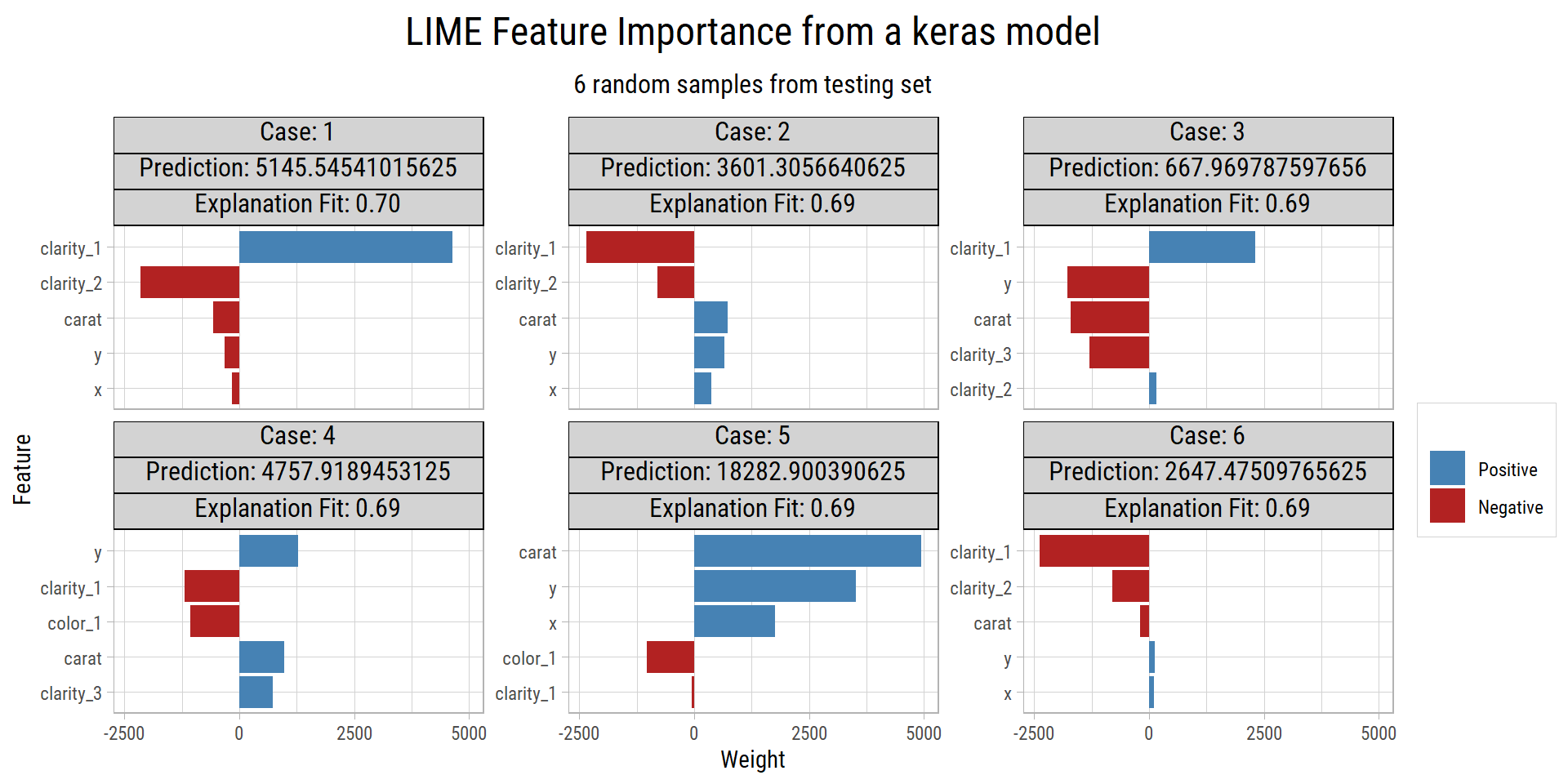
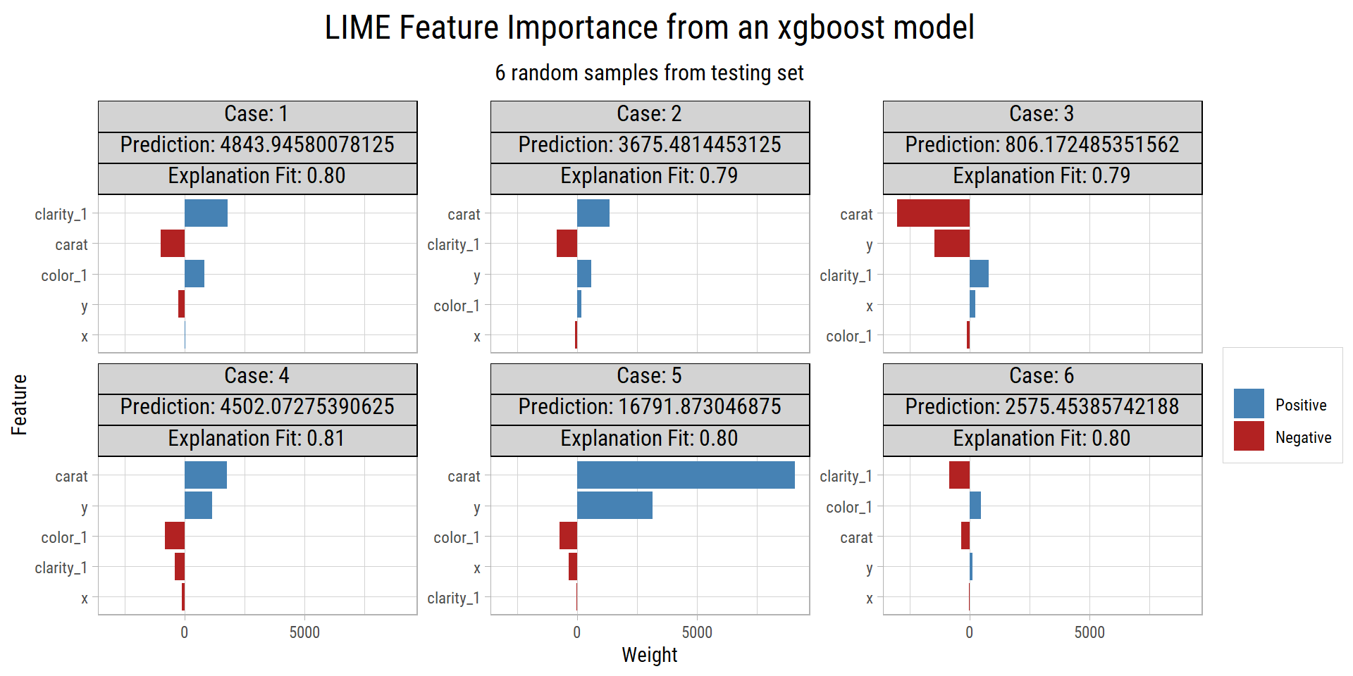
The features by importance that best explain the predictions in these 6 random samples are carat, clarity, color, x and y.
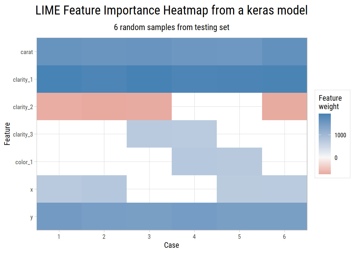
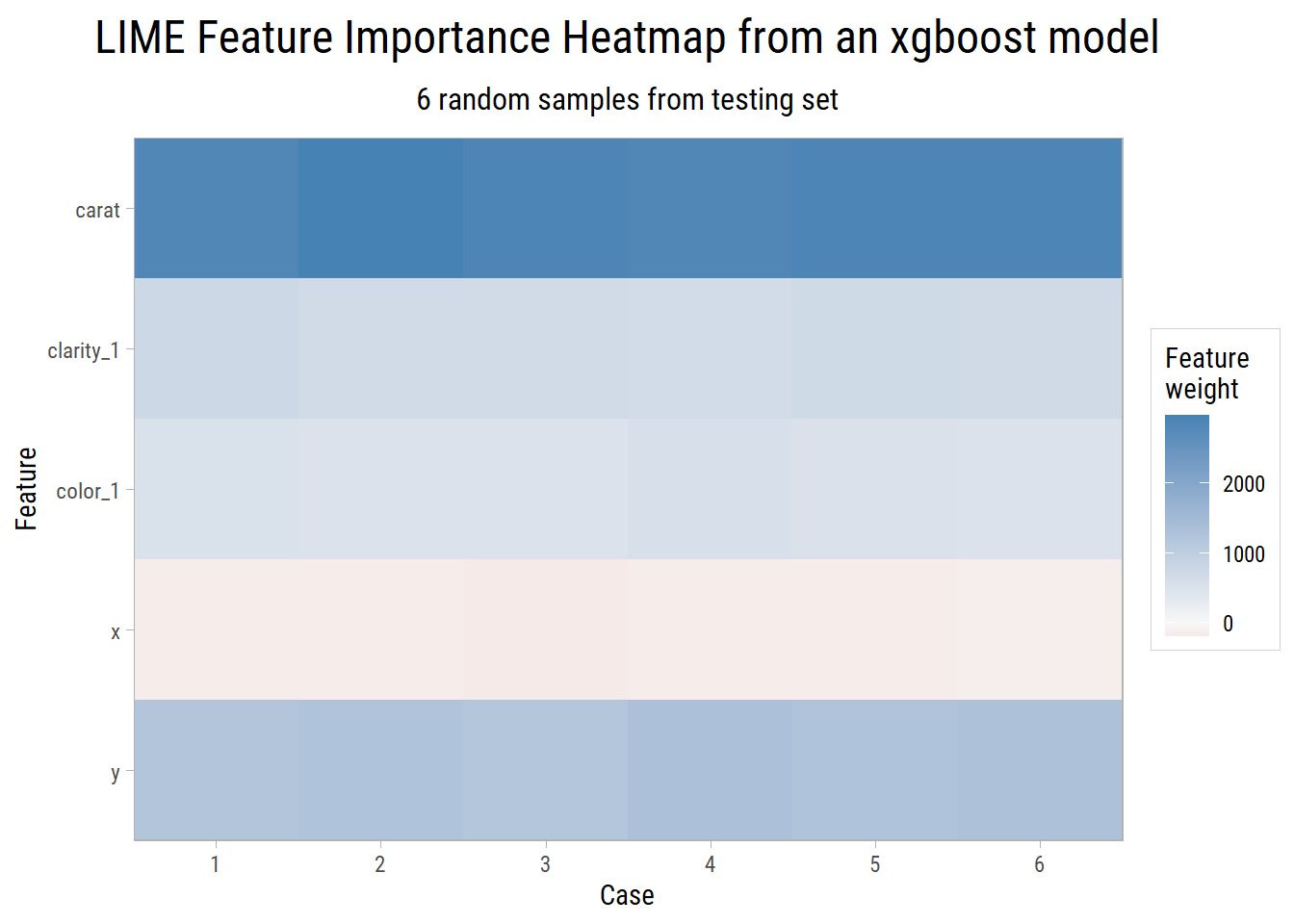
We know that x and y are co-linear with carat, which is why it is good practice to remove any redundant features from the training data before applying any machine learning algorithm. We find the model with the best metrics turns out to be the one using carat, clarity and color.
Actual v/s Predicted
Finally, here are the scatterplots of actual v/s predicted price from the best model on the testing set, using the 3 regression methods:
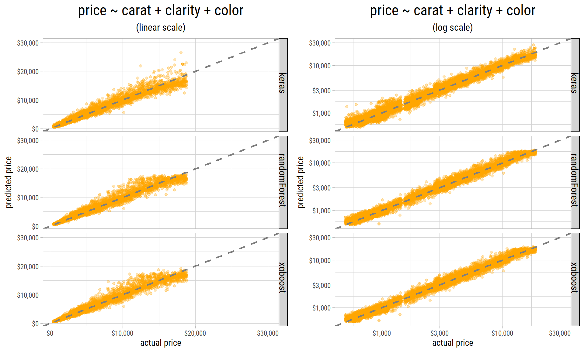
The scatterplots are shown with both linear and logarithmic axes. Even though the results from all the 3 methods have roughly similar r-squared and rmse values, we can see predicted prices from keras have more dispersion than the two decision-tree methods at the higher end. The decision-tree based methods appear do a better job of predicting prices at the lower end with lesser dispersion.
As in the case with linear models, the variance in predicted diamond prices increases with price. But unlike linear models, the non-linear models do not produce extreme outliers in predicted prices. So, not only do non-linear methods do a fantastic job in inferring the relationships between price and its predictors, they also predict prices within a reasonable range.
Summary
- All the 3 non-linear regression methods can infer the complex relationship between
price,caratand other predictors, without the need for feature engineering. - Exploratory Data Analysis is useful in removing the redundant features from the training dataset, resulting in both faster execution, as well as much better metrics.
- In terms of time taken to train the models,
kerasneural network models execute the fastest by virtue of being able to use GPUs. - Among the decision-tree based methods,
xgboostmodels train much faster thanrandomForestmodels. - Multiple CPUs can be used to run
randomForestandxgboostmethods. RAM is the only limiting constraint, when trained on a local machine.