Diamonds - Part 2 - A cut above - Building Linear Models
In a previous post in this series, we did an exploratory data analysis of the diamonds dataset and found that carat, x, y, z were strongly correlated with price. To some extent, clarity also appeared to provide some predictive ability.
In this post, we will build linear models and see how well they predict the price of diamonds.
Before we do any transformations, feature engineering or feature selections for our model, let’s see what kind of results we get from a base linear model, that uses all the features to predict price:
Call:
lm(formula = price ~ ., data = diamonds)

Residuals:
   Min     1Q Median     3Q    Max
-21376   -592   -183    376  10694

Coefficients:
            Estimate Std. Error t value             Pr(>|t|)
(Intercept)  5753.76     396.63   14.51 < 0.0000000000000002 ***
carat       11256.98      48.63  231.49 < 0.0000000000000002 ***
cut.L         584.46      22.48   26.00 < 0.0000000000000002 ***
cut.Q        -301.91      17.99  -16.78 < 0.0000000000000002 ***
cut.C         148.03      15.48    9.56 < 0.0000000000000002 ***
cut^4         -20.79      12.38   -1.68               0.0929 .
color.L     -1952.16      17.34 -112.57 < 0.0000000000000002 ***
color.Q      -672.05      15.78  -42.60 < 0.0000000000000002 ***
color.C      -165.28      14.72  -11.22 < 0.0000000000000002 ***
color^4        38.20      13.53    2.82               0.0047 **
color^5       -95.79      12.78   -7.50    0.000000000000066 ***
color^6       -48.47      11.61   -4.17    0.000030090737193 ***
clarity.L    4097.43      30.26  135.41 < 0.0000000000000002 ***
clarity.Q   -1925.00      28.23  -68.20 < 0.0000000000000002 ***
clarity.C     982.20      24.15   40.67 < 0.0000000000000002 ***
clarity^4    -364.92      19.29  -18.92 < 0.0000000000000002 ***
clarity^5     233.56      15.75   14.83 < 0.0000000000000002 ***
clarity^6       6.88      13.72    0.50               0.6157
clarity^7      90.64      12.10    7.49    0.000000000000071 ***
depth         -63.81       4.53  -14.07 < 0.0000000000000002 ***
table         -26.47       2.91   -9.09 < 0.0000000000000002 ***
x           -1008.26      32.90  -30.65 < 0.0000000000000002 ***
y               9.61      19.33    0.50               0.6192
z             -50.12      33.49   -1.50               0.1345
---
Signif. codes:  0 '***' 0.001 '**' 0.01 '*' 0.05 '.' 0.1 ' ' 1

Residual standard error: 1130 on 53916 degrees of freedom
Multiple R-squared:  0.92,  Adjusted R-squared:  0.92
F-statistic: 2.69e+04 on 23 and 53916 DF,  p-value: <0.0000000000000002
# A tibble: 3 x 3
.metric .estimator .estimate
<chr> <chr> <dbl>
1 rmse standard 1130.
2 rsq standard 0.920
3 mae standard 740. The model summary shows it is an overfitted model. Among other things, we know that depth and table have no impact on price, yet these are shown to be highly significant. Root Mean Squared Error (rmse) and other metrics are also shown above.
Let’s make a plot of actual v/s predicted prices to visualize how well this base model performs.
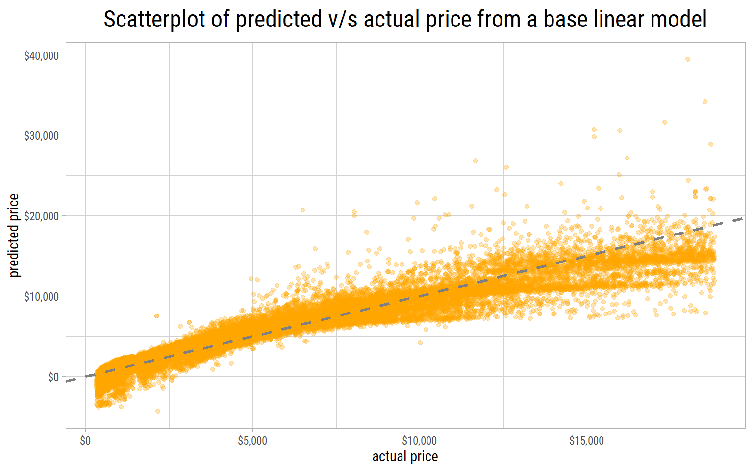
If the predictions are good, the points should lie close to a straight line drawn at 45 degrees. We can see this base model does a poor job of predicting prices. Worst of all, the model predicts negative prices on the lower end.
It shows that price has to be log transformed to avoid these absurdities.
Feature Engineering
We know the price of a diamond is strongly correlated with its size. All things equal, the larger the diamond, the greater its price.
As a first approximation, we can assume a diamond is a cuboid with dimensions x, y and z. Then, we can compute its volume as x * y * z.
As these 3 dimensions are highly correlated, we can compute a geometrical average dimension by taking the cube root of volume, and retain a linear relationship with log(price).
Another way to calculate an average dimension is by using high school chemistry. Mass, volume and density are related to each other by the equation:
$ density = mass/volume $
We can find out that 1 carat = 0.2 gms. Dividing by the density of diamond (3.51 gms/cc) would give us its volume in cc, which could be converted to a geometrical average dimension by taking the cube root.
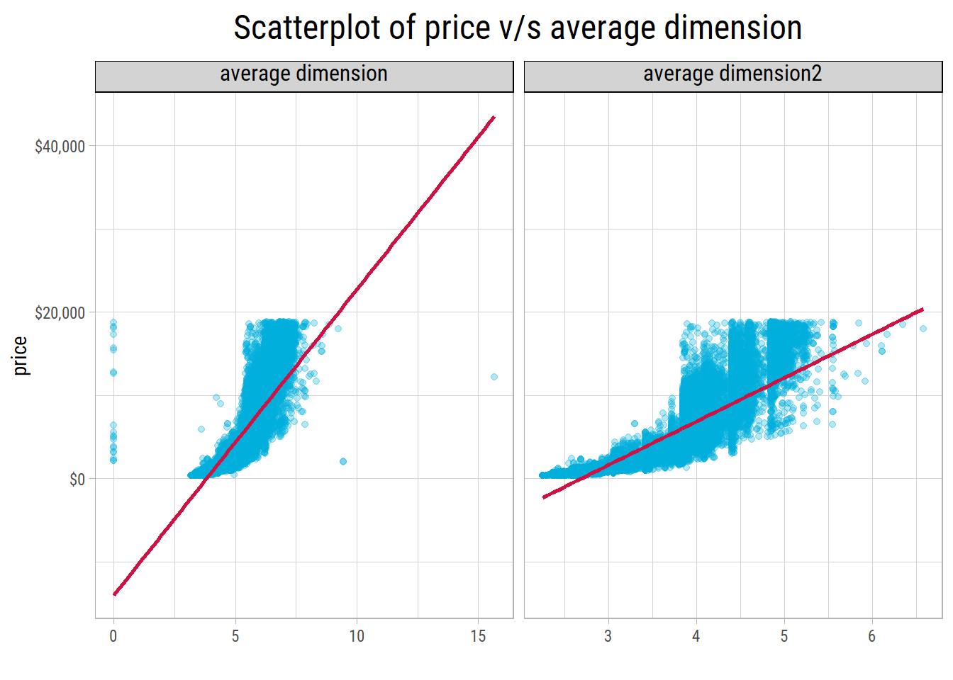
Even though both methods yield similar results, we could see that the density method results in a narrower range. But which method would be more robust?
Keep in mind there are 20 z values that are 0. In 7 of these records both x and y are 0 too, which means these values were not recorded reliably.
# A tibble: 20 x 10
   carat cut       color clarity depth table price     x     y     z
   <dbl> <ord>     <ord> <ord>   <dbl> <dbl> <int> <dbl> <dbl> <dbl>
 1  1    Premium   G     SI2      59.1    59  3142  6.55  6.48     0
 2  1.01 Premium   H     I1       58.1    59  3167  6.66  6.6      0
 3  1.1  Premium   G     SI2      63      59  3696  6.5   6.47     0
 4  1.01 Premium   F     SI2      59.2    58  3837  6.5   6.47     0
 5  1.5  Good      G     I1       64      61  4731  7.15  7.04     0
 6  1.07 Ideal     F     SI2      61.6    56  4954  0     6.62     0
 7  1    Very Good H     VS2      63.3    53  5139  0     0        0
 8  1.15 Ideal     G     VS2      59.2    56  5564  6.88  6.83     0
 9  1.14 Fair      G     VS1      57.5    67  6381  0     0        0
10  2.18 Premium   H     SI2      59.4    61 12631  8.49  8.45     0
11  1.56 Ideal     G     VS2      62.2    54 12800  0     0        0
12  2.25 Premium   I     SI1      61.3    58 15397  8.52  8.42     0
13  1.2  Premium   D     VVS1     62.1    59 15686  0     0        0
14  2.2  Premium   H     SI1      61.2    59 17265  8.42  8.37     0
15  2.25 Premium   H     SI2      62.8    59 18034  0     0        0
16  2.02 Premium   H     VS2      62.7    53 18207  8.02  7.95     0
17  2.8  Good      G     SI2      63.8    58 18788  8.9   8.85     0
18  0.71 Good      F     SI2      64.1    60  2130  0     0        0
19  0.71 Good      F     SI2      64.1    60  2130  0     0        0
20  1.12 Premium   G     I1       60.4    59  2383  6.71  6.67     0
In all of these records, the carat values were recorded reliably and are probably more accurate than the dimensions.
Hence, we might prefer the density method of generating this feature.
Furthermore, since density is a constant, dividing by a constant to calculate volume isn’t really necessary. Instead, a cube root transformation could be applied to carat itself for the purposes of predictive modelling that would result in a linear relationship between \(log(price)\) and \(carat^{1/3}\).
It is the reason why we’re fitting a linear model because the model is linear in its parameters.
Training Linear Models
Here are the steps for building linear models and computing metrics:
- Partition the dataset into training and testing sets in the proportion 75% and 25% respectively.
- Since
clarityis one of the main predictors, stratify the partitioning byclarity, so both training and testing sets have the same distributions of this feature. - Fit a linear model with the training set.
- Make predictions on the testing set and determine model metrics.
- Wrap all the steps above inside a function in which the model formula and a seed could be passed. Since the seed determines the random partitioning, it helps to minimize vagaries in partitioning the training and testing sets before fitting models.
- Run multiple iterations of a model with different seeds, and compute its average metrics, that would reflect the results on unseen data.
Here’s a sample split of training and testing set, stratified by clarity. As we can see, the training and testing sets have similar distributions.
dfTrain$clarity
       n  missing distinct
   40457        0        8

lowest : I1   SI2  SI1  VS2  VS1 , highest: VS2  VS1  VVS2 VVS1 IF

Value         I1   SI2   SI1   VS2   VS1  VVS2  VVS1    IF
Frequency    552  6895  9826  9222  6125  3780  2722  1335
Proportion 0.014 0.170 0.243 0.228 0.151 0.093 0.067 0.033
dfTest$clarity
n missing distinct
13483 0 8
lowest : I1 SI2 SI1 VS2 VS1 , highest: VS2 VS1 VVS2 VVS1 IF
Value I1 SI2 SI1 VS2 VS1 VVS2 VVS1 IF
Frequency 189 2299 3239 3036 2046 1286 933 455
Proportion 0.014 0.171 0.240 0.225 0.152 0.095 0.069 0.034After running 5 iterations of each model with a different seed, here are the average metrics:
# A tibble: 5 x 4
  model                                                 rmse   rsq   mae
  <chr>                                                <dbl> <dbl> <dbl>
1 log(price) ~ .                                      11055. 0.670  570.
2 log(price) ~ I(carat^(1/3))                          2893. 0.687 1039.
3 log(price) ~ I(carat^(1/3)) + clarity                2312. 0.807  881.
4 log(price) ~ I(carat^(1/3)) + clarity + color        1870. 0.870  631.
5 log(price) ~ I(carat^(1/3)) + clarity + color + cut  1848. 0.875  625.
The first model with all predictors is an overfitted one.
The model with carat, clarity and color provides the best combination of root mean squared error and r-squared, that explains the most variance.
This is our final model.
Including cut in the model has diminishing benefits, and tends to overfit the data.
Here’s the summary of our final model:
Call:
lm(formula = model_formula, data = dfTrain)

Residuals:
    Min      1Q  Median      3Q     Max
-1.6022 -0.1034  0.0145  0.1066  1.7941

Coefficients:
                Estimate Std. Error t value             Pr(>|t|)
(Intercept)     2.147009   0.004993  429.99 < 0.0000000000000002 ***
I(carat^(1/3))  6.246412   0.005365 1164.27 < 0.0000000000000002 ***
clarity.L       0.922295   0.005036  183.15 < 0.0000000000000002 ***
clarity.Q      -0.295539   0.004734  -62.43 < 0.0000000000000002 ***
clarity.C       0.166979   0.004068   41.05 < 0.0000000000000002 ***
clarity^4      -0.068591   0.003260  -21.04 < 0.0000000000000002 ***
clarity^5       0.032833   0.002669   12.30 < 0.0000000000000002 ***
clarity^6      -0.001904   0.002325   -0.82              0.41288
clarity^7       0.025508   0.002049   12.45 < 0.0000000000000002 ***
color.L        -0.488882   0.002927 -167.05 < 0.0000000000000002 ***
color.Q        -0.117319   0.002680  -43.78 < 0.0000000000000002 ***
color.C        -0.012230   0.002497   -4.90           0.00000098 ***
color^4         0.019007   0.002288    8.31 < 0.0000000000000002 ***
color^5        -0.008110   0.002159   -3.76              0.00017 ***
color^6        -0.000396   0.001967   -0.20              0.84055
---
Signif. codes:  0 '***' 0.001 '**' 0.01 '*' 0.05 '.' 0.1 ' ' 1

Residual standard error: 0.166 on 40442 degrees of freedom
Multiple R-squared:  0.973, Adjusted R-squared:  0.973
F-statistic: 1.05e+05 on 14 and 40442 DF,  p-value: <0.0000000000000002
Here’s a scatterplot of actual v/s predicted log(price) from our final model on the testing set:
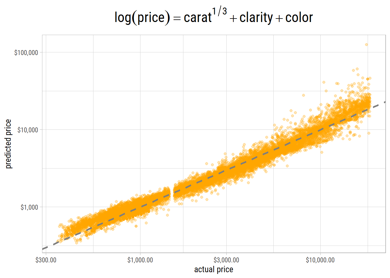
The points lie close to the 45 degress line. However, on the high end, there are many outliers where actual and predicted values have very high variance. Nevertheless, this is as good as it gets.