Ames Housing - Part 2 - Building Models
In a previous post in this series, we did an exploratory data analysis of the Ames Housing dataset.
In this post, we will build linear and non-linear models and see how well they predict the SalePrice of properties.
Evaluation Criteria
Root-Mean-Squared-Error (RMSE) between the logarithm of the predicted value and the logarithm of the observed SalePrice will be our evaluation criteria. Taking the log ensures that errors in predicting expensive and cheap houses will affect the result equally.
Steps for Building Models
Here are the steps for building models and determining the best hyperparameter combinations by K-fold cross validation:
- Partition the training dataset into model training and validation sets. Use stratified sampling such that each partition has a similar distribution of the target variable -
SalePrice. - Define linear and non-linear models.
- For each model, create a grid of hyperparameter combinations that are equally spaced.
- For each hyperparameter combination, fit a model on the training set and make predictions on the validation set. Repeat the process for all folds.
- Determine root mean squared errors (RMSE) and choose the best hyperparameter combination that corresponds to the minimum RMSE.
- Train each model with its best hyperparameter combination on the entire training set.
- Calculate RMSE of the each finalized model on the testing set.
- Finally, choose the best model that gives the least RMSE.
Partitioning Training Data
We split the training data into 4 folds. Within each fold, 75% of the data is used for training models and 25% for validating the predicted values against the actual values.
Let’s look at the distribution of the target variable across all folds:
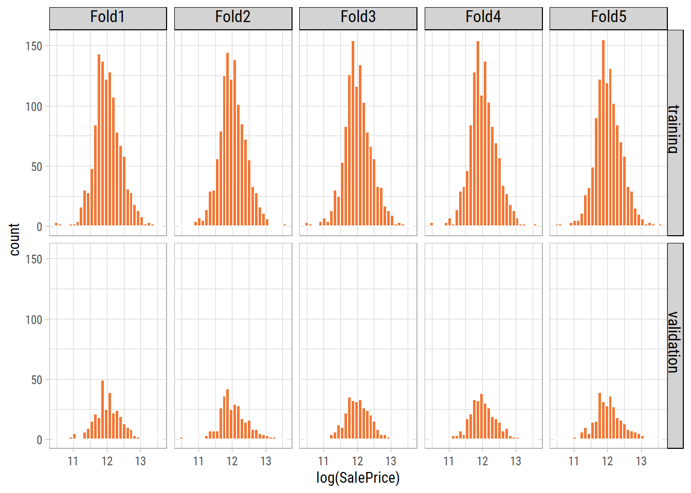
By using stratified sampling, we ensure that the training and validation distributions of the target variable are similar.
Linear Models
Ordinary Least Squares Regression
Before creating any new features or indulging in more complex modelling methods, we will cross validate a simple linear model on the training data to establish a benchmark. If more complex approaches do not have a significant improvement in the model validation metrics, then they are not worthwhile to be pursued.
Linear Regression Model Specification (regression)

Computational engine: lm
What’s notable?
- After training a linear model on all predictors, we get an RMSE of 0.1468.
- This is the simplest and fastest model with no hyperparameters to tune.
Regularized Linear Model
We will use glmnet that uses LASSO and Ridge Regression with regularization. We will do a grid search of the following hyperparameters that minimize RMSE:
penalty: The total amount of regularization in the model.mixture: The proportion of L1 regularization in the model.
Linear Regression Model Specification (regression)

Main Arguments:
  penalty = tune()
  mixture = tune()

Computational engine: glmnet
Let’s take a look at the top 10 RMSE values and hyperparameter combinations:
# A tibble: 10 x 3
    penalty mixture mean_rmse
      <dbl>   <dbl>     <dbl>
 1 4.83e- 3  0.922      0.127
 2 3.79e- 2  0.0518     0.129
 3 1.36e- 3  0.659      0.132
 4 1.60e- 3  0.431      0.133
 5 3.50e- 3  0.177      0.133
 6 4.17e- 2  0.288      0.133
 7 5.67e- 4  0.970      0.133
 8 6.79e- 9  0.0193     0.138
 9 4.32e-10  0.337      0.138
10 1.95e- 6  0.991      0.138
What’s notable?
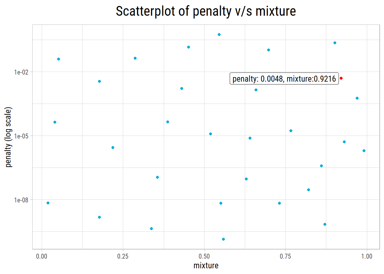
- After hyperparameter tuning with cross validation,
glmnetgives the best RMSE of 0.127 with penalty = 0.0048 and mixture = 0.9216. - It is a significant improvement over Ordinary Least Squares regression that had an RMSE of 0.1468.
glmnetcross validation takes under a minute to execute.- But the presence of outliers can significantly affect its performance.
Here a plot of the glmnet hyperparameter grid along with the best hyperparameter combination:
Non-linear Models
Next, we will train a couple of tree-based algorithms, which are not very sensitive to outliers and skewed data.
randomForest
In each ensemble, we have 1000 trees and do a grid search of the following hyperparameters:
mtry: The number of predictors to randomly sample at each split.min_n: The minimum number of data points in a node required to further split the node.
Random Forest Model Specification (regression)

Main Arguments:
  mtry = tune()
  trees = 1000
  min_n = tune()

Engine-Specific Arguments:
  objective = reg:squarederror

Computational engine: randomForest
Let’s take a look at the top 10 RMSE values and hyperparameter combinations:
# A tibble: 10 x 3
   min_n  mtry mean_rmse
   <int> <int>     <dbl>
 1     4    85     0.134
 2     3   140     0.135
 3    14    90     0.135
 4     6    45     0.136
 5     9   138     0.136
 6    13   158     0.137
 7     9   183     0.137
 8    19    56     0.138
 9    21   130     0.138
10     5   218     0.138
What’s notable?
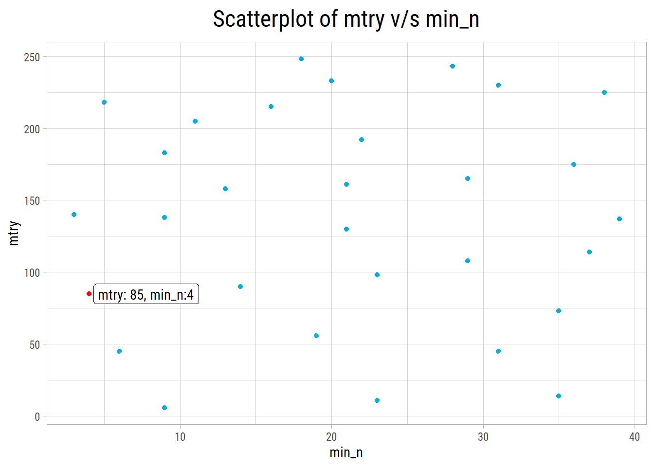
- After cross validation, we get the best RMSE of 0.134 with mtry = 85 and min_n = 4.
- This is no improvement in RMSE compared to
glmnetandrandomForestcross validation takes much longer to execute thanglmnet.
Here a plot of the randomForest hyperparameter grid along with the best hyperparameter combination:
xgboost
In each ensemble we have 1000 trees and do a grid search of the following hyperparameters:
min_n: The minimum number of data points in a node required to further split the node.tree_depth: The maximum depth or the number of splits of the tree.learn_rate: The rate at which the boosting algorithm adapts from one iteration to another.
Boosted Tree Model Specification (regression)

Main Arguments:
  trees = 1000
  min_n = tune()
  tree_depth = tune()
  learn_rate = tune()

Engine-Specific Arguments:
  objective = reg:squarederror

Computational engine: xgboost
Let’s take a look at the top 10 RMSE values and hyperparameter combinations:
# A tibble: 10 x 4
   min_n tree_depth learn_rate mean_rmse
   <int>      <int>      <dbl>     <dbl>
 1    13          3  0.0309        0.124
 2    40          4  0.0350        0.126
 3     6          8  0.0469        0.126
 4    34         15  0.0172        0.127
 5    28         10  0.0336        0.128
 6    20         14  0.00348       0.389
 7    22          7  0.000953      4.46
 8     3          2  0.000528      6.81
 9    10         12  0.000401      7.73
10    34          3  0.0000802    10.6
What’s notable?
- After cross validation, we get the best RMSE of 0.124 with min_n = 13, tree_depth = 3 and learn_rate = 0.0309.
- Gives the best RMSE compared to
glmnetandrandomForest. - However,
xgboostcross validation takes longer to execute than that ofglmnet, but is faster than that ofrandomForest
Finalizing Models
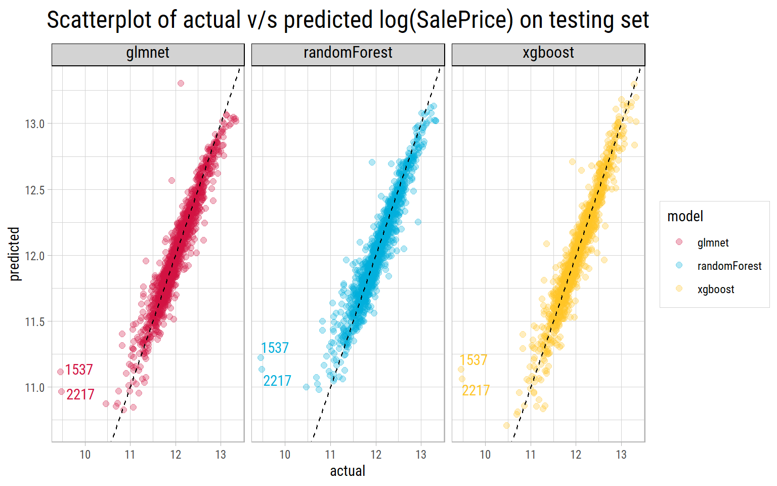
For each model, we found the combination of hyperparameters that minimize RMSE. Using those parameters, we can now train the same models on the entire training dataset. Finally, we can use the trained models to predict log(SalePrice) on the entire training set to see the actual v/s predicted log(SalePrice) results.
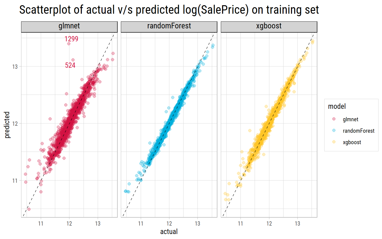
What’s notable?
- Both
randomForestandxgboostmodels do a fantastic job of predicting log(SalePrice) with the tuned parameters, as the predictions lie close to the straight line drawn at 45 degrees. - The
glmnetmodel shows a couple of outliers with Ids 524 and 1299 whose predicted values are far in excess of their actual values. Even properties whoseSalePriceis at the lower end, show a wide dispersion in prediced values. - But the true performance can only be measured on unseen testing data.
Performance on Test Data
# A tibble: 3 x 3
  model        test_rmse cv_rmse
  <chr>            <dbl>   <dbl>
1 glmnet           0.129   0.127
2 randomForest     0.139   0.134
3 xgboost          0.128   0.124
What’s notable?
- All models have similar RMSE on the unseen testing set as their cross validated RMSE, which shows the cross validation process and hyperparameters worked very well.
- Records with Ids 1537 and 2217 are outliers, as none of the models are able to predict close to actual values.
- Looking at the test RMSE, we could finalize
xgboostas the model that generalizes very well on this dataset.
Feature Importance
Even though xgboost is not as easily interpretable as a linear model, we could use variable importance plots to determine the most important features selected by the model.
Let’s take a look at the top 10 most important features of our finalized xgboost model:
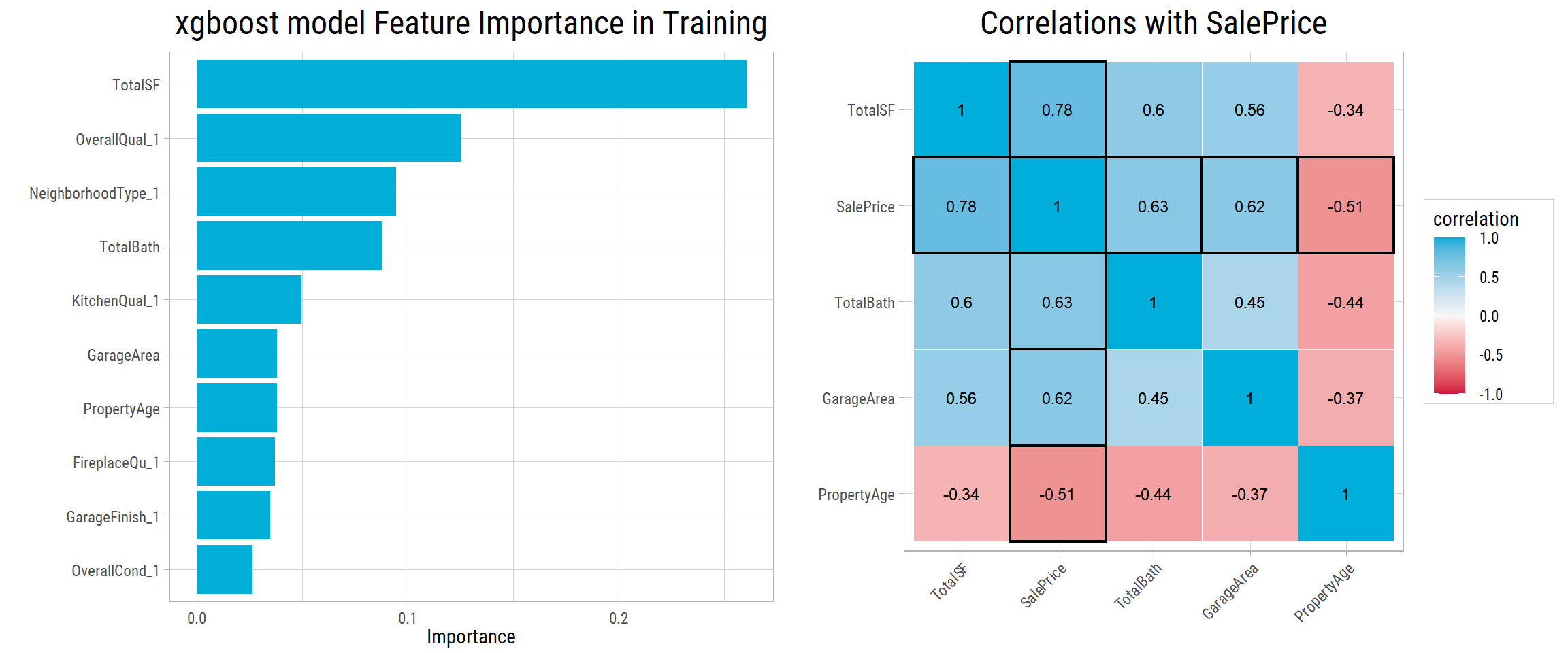
- Correlations of numerical features are plotted side-by-side. All features have a correlation of 0.5 or more with
SalePrice. - All of the top 10 features make sense. To evaluate
SalePrice, a buyer would definitely look at total square footage, overall quality, neighborhood, number of bathrooms, kitchen quality, age of property, etc. - This shows, our finalized model generalizes well and makes very reasonable choices in terms of features.
New Property Premium
Among the top 10 features by importance in our final model, most of the features like square footage, neighborhood and number of bathrooms remain the same throughout the life of the property. Quality and condition of property does change but their evaluation is mostly subjective. The only other feature that cannot be disputed to change over time is PropertyAge.
So, how would the predicted SalePrice differ if a property was newly constructed vis-a-vis the same property if it were constructed more than 30 years earlier, and all the times in between?
We could pick a couple of properties at random, change PropertyAge and see its impact on SalePrice.
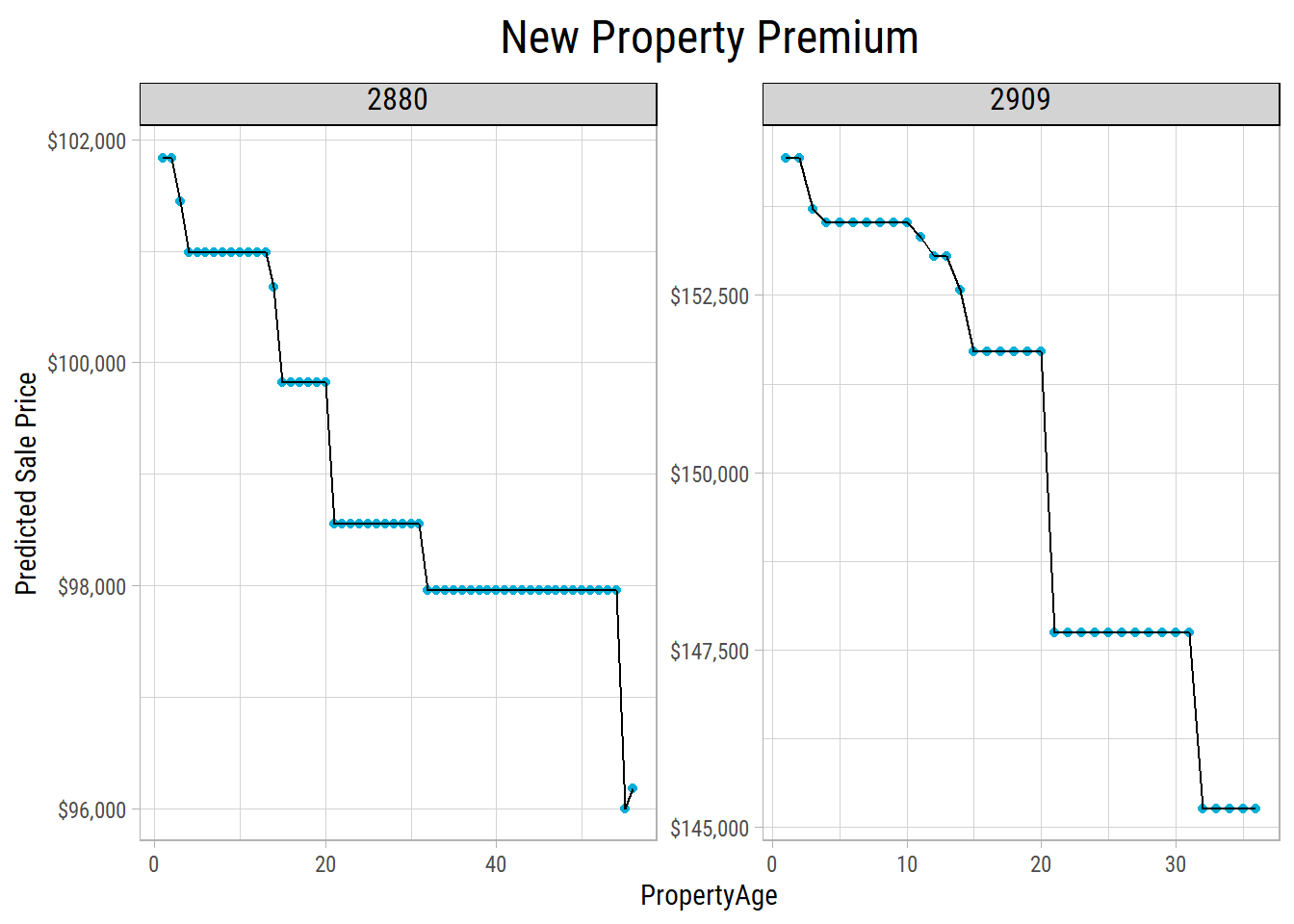
We can see there’s a small premium for a newly constructed property v/s an older property of the same build, quality and condition. This premium isn’t very much in a place like Ames, IA but we’d reckon it would be much higher in a larger metropolitan city.