How would you bet? Lessons from a Biased Coin Flipping Experiment
Recently I listened to a podcast featuring Victor Haghani of Elm Partners, who described a fascinating coin-flipping experiment. The experiment was designed to be played for 30 minutes by participants in groups of 2-15 in university classrooms or office conference rooms, without consulting each other or the internet or other resources. To conduct the experiment, a custom web app was built for placing bets on a simulated coin with a 60% chance of coming up heads. Participants used their personal laptops or work computers to play. They were offered a stake of \(\$25\) to begin, with a promise of a check worth the final balance (subject to a caveat) in their game account. No out-of-pocket betting or any gimmicks. But they had to agree to remain in the room for 30 minutes.
Even though the experiment in no longer active, the game URL is still active. Before reading any further, I strongly encourage readers to play the game and decide how they would bet and what outcomes they should expect? SPOILERS AHEAD
What would be an optimal betting strategy?
The details of the experiment are described in a paper that would be very accessible to anyone with a rudimentary understanding of probability.
The probability of heads is reported to be 60%, which means that if the game’s virtual coin is flipped sufficiently large number of times, the number of heads should converge to 60% of the total outcomes. Since each flip is independent of all prior flips, there is a positive expectancy in betting on heads only. The expected gain in betting an amount \(x\) on heads is \(0.6x - 0.4x = 0.2x\)
But how should one bet? Intuitively it is apparent that betting too large would be counter-productive because if we lose, the balance would deplete quickly. A string of consecutive losses would quickly lead to bankruptcy. On the other hand, betting too little isn’t going to be very productive either, even though we know the odds of betting on heads are favorable.
So, somewhere along the spectrum between betting too little or too large, there is an optimal betting strategy. In 1955 John Kelly working at Bell Labs published a formula that showed how to maximize wealth while betting on games with favorable odds. Even though this formula has been known to professional gamblers for decades, to my knowledge, it is not a part of any high school or undergraduate curriculum on probability and statistics. I know this personally, having a background in science and engineering.
When the Kelly formula is applied to a game like this with binary (heads/tails) outcomes, it suggests betting a constant fraction of the existing balance, denoted by \(2*p - 1\), where p is the probability of the favorable outcome. Clearly, the outcome would be favorable only if p > 0.5.
Given that the probability of heads in this game is 0.6, the optimal bet size is \(2*0.6-1 = 0.2\) or 20% of the existing balance at each flip. This optimality could be demonstrated by simulation.
In the original experiment, 61 participants flipped virtual coins 7253 times. So during the course of a 30 min game, a virtual coin was flipped ~ 120 times on average.
I generated a sample set of 1000 games. In each game, a virtual coin is flipped 120 times with a 0.6 probability of getting heads.
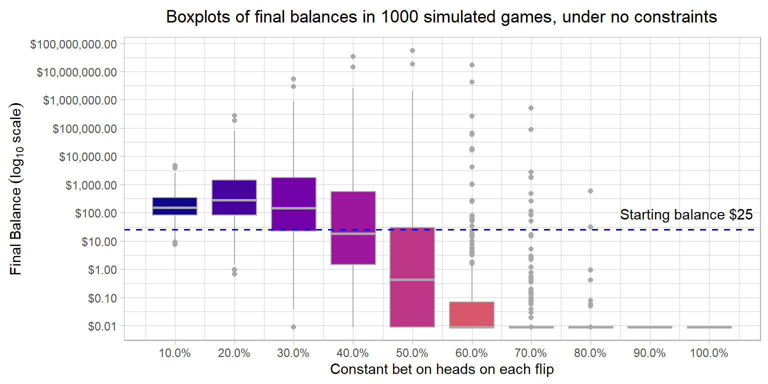
Assuming there are no constraints in the game and the upside is unbounded, the boxplots show the range of outcomes resulting from a constant percentage bet on heads on each flip.
Few things stand out from this plot:
Since the lowest balance could only be 0 and the maximum is unbounded, the median provides a better measure of the central tendency of the betting outcomes. The mean is highly skewed by extreme outcomes on the upside. The median provides a balance between those who got extremely lucky and those who weren’t so much. The median balance is the highest while maintaining a constant 20% bet, which is exactly what the Kelly formula suggests.
If you played the game and didn’t discover the maximum payout, it should be very evident looking at this plot that the game can’t be offered practically without an upper limit. In this sample, the final balance reaches ~ \(\$55\) million in a game with 120 flips betting 50% on heads, even though this would be far from an ideal betting strategy. In theory, if someone got extremely lucky they could flip 120 heads in succession and bet 100% each time to get a final balance of \(25*1.2^{120} = \$79.4\) billion; although this would be extremely unlikely.
While betting 40% of the balance, odds are low that you would make more than the starting balance of \(\$25\)
While betting 60% or more of the balance, you are almost guaranteed to end up below the starting balance of \(\$25\)
While betting 80% or more of the balance, you are almost guaranteed to go bankrupt
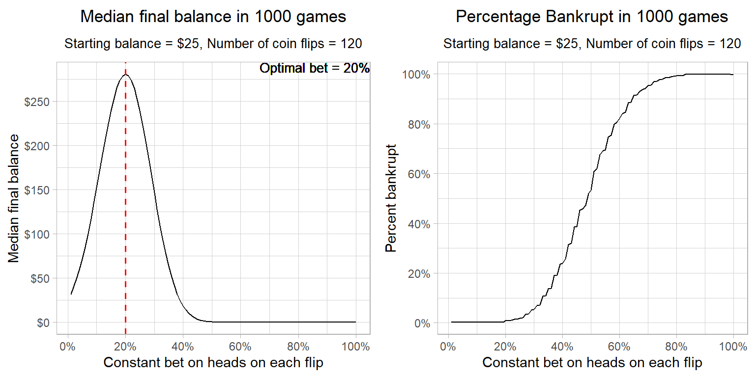
The plots of median final balance and the percentage of games which lead to bankruptcy at each constant proportional bet are shown below, These plots make it clear why the Kelly formula provides the optimal betting strategy. The risk with respect to reward is well-balanced.
The Kelly formula assumes log utility of wealth. With a constant proportional bet of 20% with a 60% chance of heads, the expected utility for each flip is:
\(0.6*log(1.2) + 0.4*log(0.8) = 0.020136\), which means that each flip gives a dollar equivalent increase in utility of \(exp(0.020136)\) =1.0203401 or ~ 2%
So, 120 flips starting at \(\$25\), leads to \(\$25*(1.0203401^{120}) = \$280.1\)
Alternatively, in 120 flips, if 60% or 72 were heads, the median outcome could be calculated by \(\$25*(1.2^{72})*(0.8^{48}) = \$280.1\)
Both of these values correspond to the peak of the median final balance determined from simulation. The median values for other constant proportional bets could be calculated in the same manner.
Simulating the game play
If you’ve read this far, you understand this game can’t be offered without an upper limit on the final payout. If you played the game and bet wisely or were just plain lucky, you would’ve discovered that the maximum payout is \(\$250\). So the objective changes mid-game from growing to preserving existing balance. Once the maximum payout balance is reached, it is foolhardy to keep betting large sums no matter what betting strategy you have chosen.
Secondly, the UI design of the app doesn’t have a mechanism to choose a constant percentage bet level. So, if you were following a systematic betting strategy like Kelly, then you would have to do mental calculations to determine the exact dollar amount. While this is not hard to do, I believe most people would just round up or down to the nearest dollar amount. Also it takes less time to input a whole dollar amount than dollars and cents. So even though the minimum bet size in the game is 1 cent, effectively it would be \(\$1\).
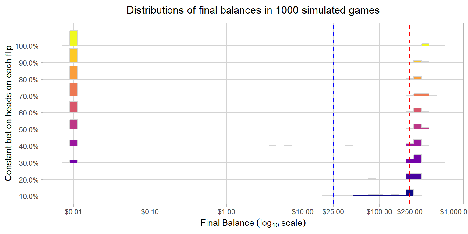
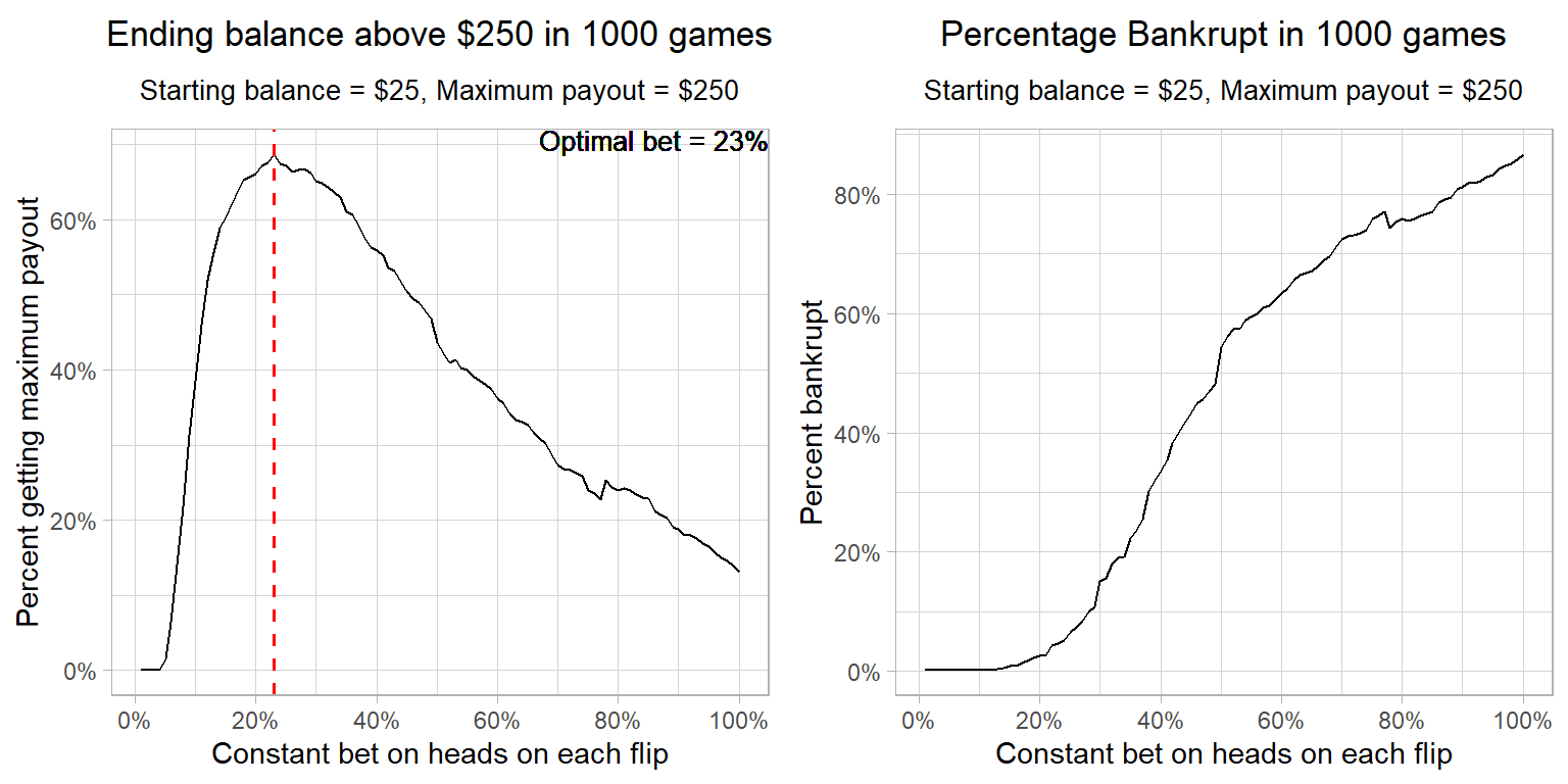
Under these constraints and assumptions, the plot shows bimodal distributions at all bet levels. During the game, the objective changes to maximizing the chances of ending a game above the maximum payout of \(\$250\). Here we can see that the Kelly formula turned out to be a close approximation to optimal, even though the optimal level is determined only in hindsight. Fewer bankruptcies result at higher bet levels than in unconstrained games. I made the assumption that the participants who got lucky early on betting big, decided to bet just \(\$1\) on all subsequent bets after discovering the maximum payout.
How did the participants do in the experiment?
Not very well to say the least. There’s an excellent discussion in the paper, but here are the salient points:
- Only 21% of the participants reached the maximum payout of \(\$250\)
- 51% of the participants neither went bust nor reached the maximum payout. Their average final balance was \(\$75\)
- 33% of the participants ended up below the starting balance of \(\$25\)
- 28% of the participants went bust and received no payout
- Average payout across all participants was \(\$91\)
- Only 5 among the 61 participants had heard of the Kelly criterion. Out of those, only 1 managed to barely double his stake while the other broke even after 100 flips
Betting Patterns
Betting patterns were found to be quite erratic.
- 18 participants bet all-in on one flip
- Some bet too small and then too big
- Many participants adopted a Martingale strategy where the losing bets are doubled up to recover past losses
- Some bet small constant wagers to minimize chances of ruin and end up with a positive balance
- 41 participants (67%!!) bet on tails at some point during the game play. 29 of them bet on tails 5 or more times
Despite how terrible some of these betting strategies may have been, hitting the maximum payout limit might have saved some of them from ending up bankrupt. Well, assuming these participants were not foolish enough to keep betting high after knowing they couldn’t get more than \(\$250\).
Let’s see how some of these betting patterns work in simulation.
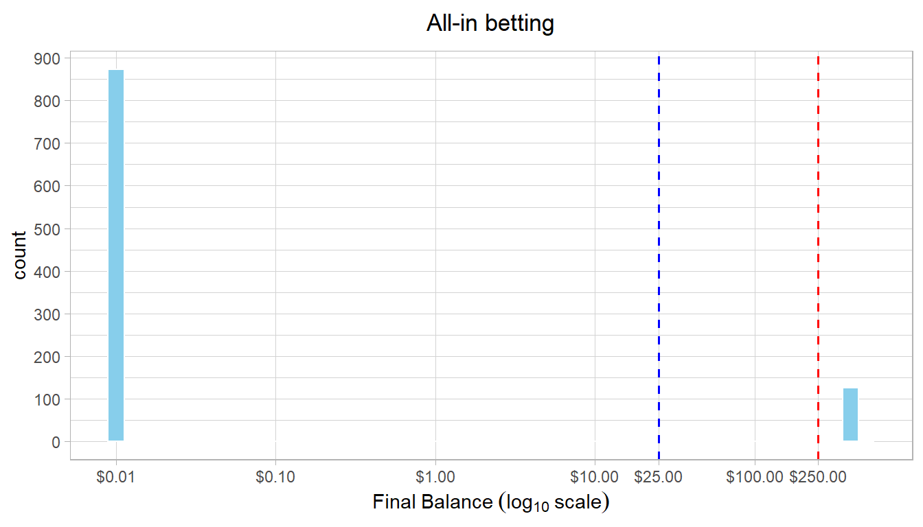
All-in Betting
18 out of 61 participants reportedly bet 100% on a single flip. Assuming they continued this betting pattern, majority of these participants would’ve lost everything after their second bet. Those who reached the maximum payout would’ve had to win first 4 flips in succession. Assuming they kept their wits beyond that point, only 13% of such participants would’ve ended up with a balance of \(\$250\) or more.
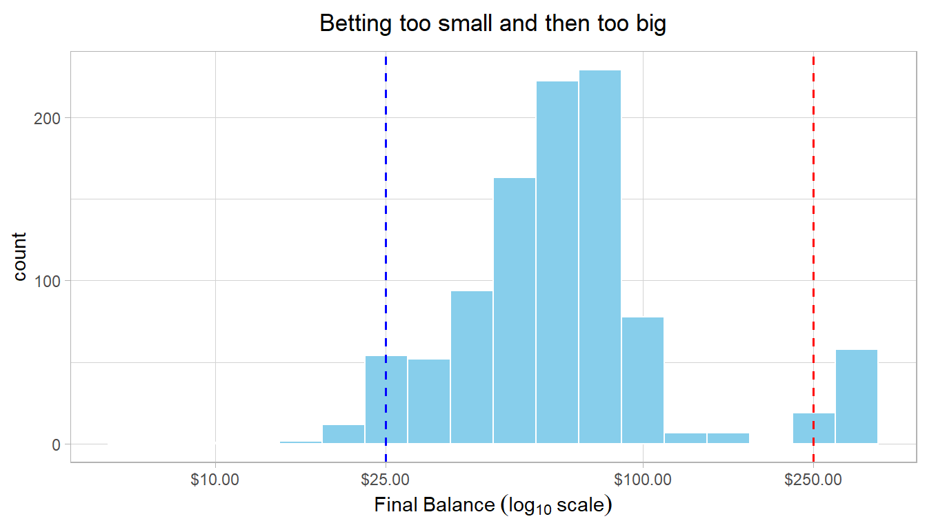
Betting too small and then too big
Some participants bet too small and then too big. It appears they were over-cautious at first, but when they built a sizeable balance, they threw caution to the wind. Some form of wealth effect or house money effect came into play.
To simulate this strategy, I assumed such participants bet 5% until they accumulated a balance of \(\$100\), after which they started betting 30%. If their balance fell below \(\$100\) again, they got spooked and adopted the 5% conservative bet again.
The simulated results are quite interesting. Although none of the participants would’ve been bankrupted (assuming they adopted the ultra safe 5% bets when their balance was lower), only ~ 10% of them would’ve made \(\$250\) or more.
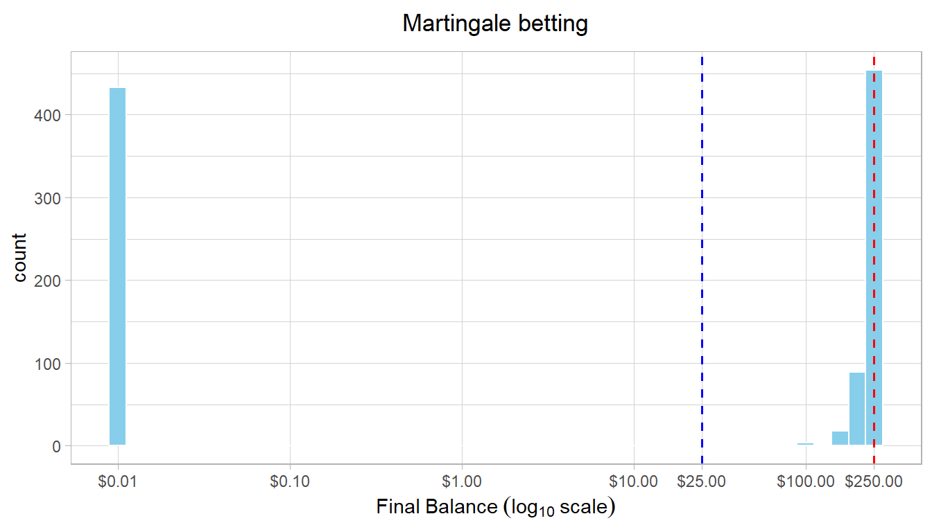
Martingale betting
Martingale bettors keep doubling up their bets after every loss. For instance, if they bet \(\$2\) and lost, their next bet would be \(\$4\), and the next one \(\$8\) if they lost again. Their idea is to recover the former loss(es) and make profits equal to the original stake. Most often this strategy starts with betting small and doubles up on the previous bet even in successive losses. This idea mostly stems from gambler’s fallacy. So if a Martingale bettor was betting on heads but the coin flipped tails several times in succession, their belief is the next flip would be heads and they’ll recover everything they’ve lost thus far. After all mean reversion should come into play, right?.
But mean reversion could take much longer to manifest. The coin has no memory of the past flips. Every flip is independent of the prior flips. Even with a biased coin like in this game, it could very well happen that it flips tails 20 times in succession and then flips heads 30 times in succession. The probability of heads converges to 0.6 only in the long run. After losing 20 bets in succession starting with \(\$1\), a Martingale bettor would need to bet ~ $1.05 million to recover past losses.
To simulate this betting strategy, I assumed a minimum bet size of \(\$1\) as long as the balance is \(\$25\) or lower i.e. 4% to start. The minimum bet is readjusted proportionally as the balance increases or decreases in multiples of \(\$25\). So it goes up to \(\$2\) when the balance is above \(\$50\) and \(\$4\) when the balance is above \(\$100\). The previous losing bet is doubled up in succession.
The simulated results show 42% of the bettors going bankrupt with this strategy. Only 38% of the bettors would’ve ended up with \(\$250\) or more.
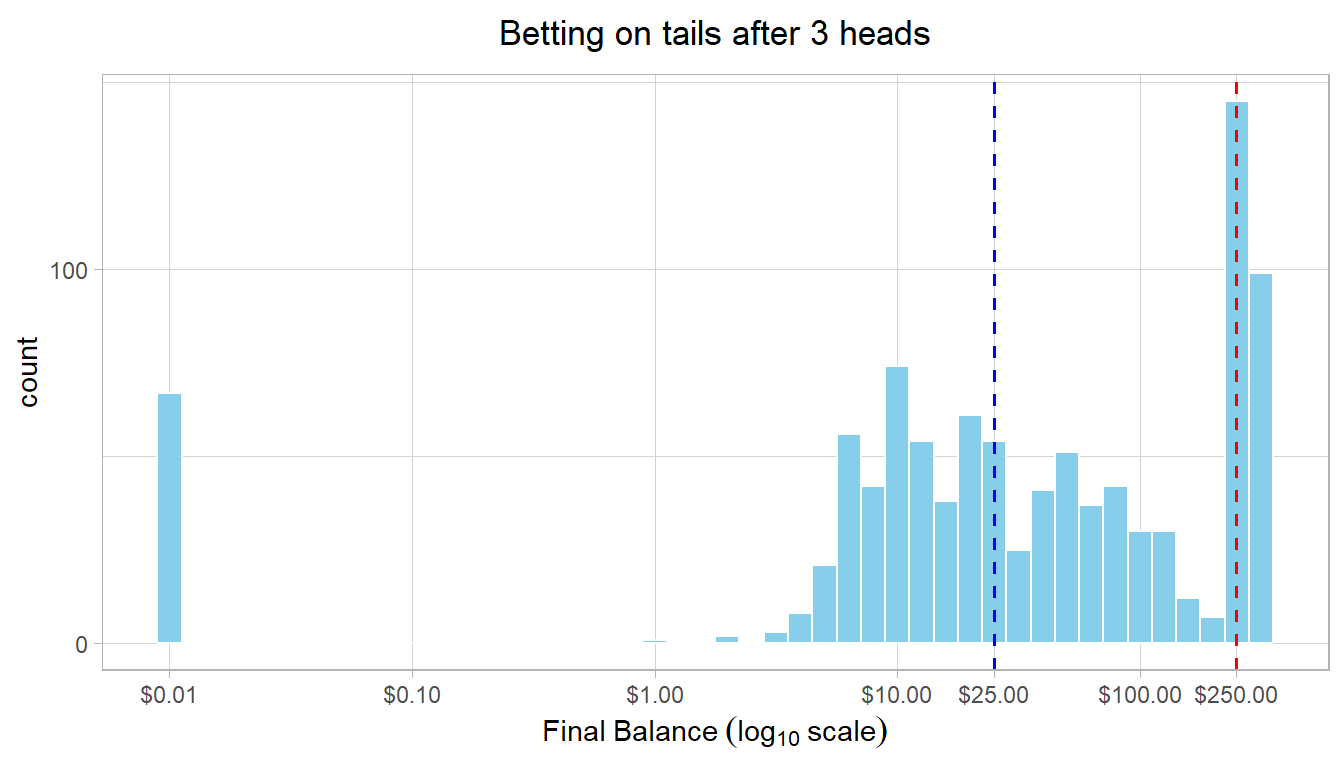
Betting on tails
There were 41 participants who bet on tails at some point during the game. 29 of them bet on tails more than 5 times in the game. 13 of them bet on tails more than 25% of the time. These participants were more likely to make that bet after a string of consecutive heads. As the authors state in the paper “…some combination of the illusion of control, law of small number bias, gambler’s fallacy or hot hand fallacy was at work”.
Let’s assume, these participants bet on heads, until a string of ‘X’ heads, after which they kept betting on tails until they got one, after which they bet on heads again repeating the same process. What would be the value of ‘X’ for the participants to bet on tails more than 25% of the time? We could get a sense from the simulated game data.
Heads_Threshold_2 Heads_Threshold_3 Heads_Threshold_4 Heads_Threshold_5 Heads_Threshold_6
             0.35              0.21              0.12              0.07              0.04
It turns out most of these participants were expecting tails after a string of 3 or more heads. Assuming they followed this heuristic, even while making the optimal 20% bet, the simulated results show ~ 7% of the participants going bankrupt and only 25% of them ending up with \(\$250\).
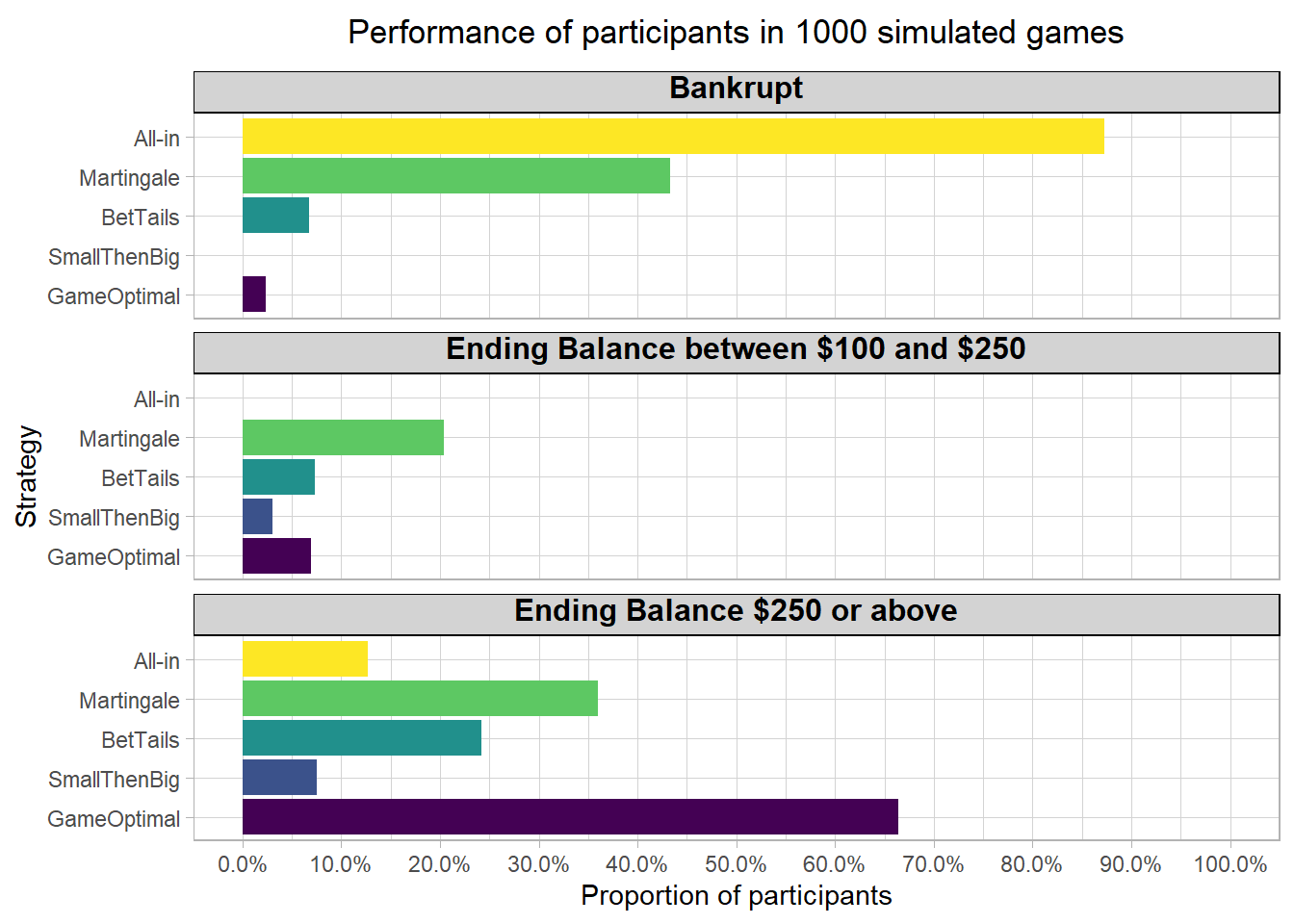
Comparison of Betting Strategies
The plot below shows the performance of the betting strategies modelled above, with respect to a game optimal strategy of betting 20% of the balance. Most of them end up with a much higher proportion of participants going bankrupt in the game. No strategy comes anywhere close to the game optimal strategy, when it comes to the number of participants reaching the maximum payout offered in the game.
In fact, discovering the maximum payout of \(\$250\) would’ve helped some of the participants employing these wayward betting strategies into adopting more conservative approaches in the latter part of their game. But if the game was designed to payout a fraction of the final balance, some more interesting outcomes might emerge. For instance, the maximum balance in the game could be raised to 2500 and the actual payout could be a tenth of that (\(\$250\) still). The evidence from simulated results suggests the outcomes in that case to be much worse.
How did I play the game?
To be sure, I was not a part of the cohort of 61 participants who played this game in person and were paid for participation. The game URL is still active, even though there’s no actual payout offered any more. I found it after listening to the podcast and reading the paper. So, unfortunately I already knew the optimal strategy before trying. In my gameplay, I reached the maximum payout by the 16th minute. I ended up with a balance of \(\$270\), flipping the virtual coin a total of 122 times.
I did however, get some loved ones to play the game uninformed and then tell me their betting strategies. In a sample of n = 4, they reported everything from Martingale betting, betting 10 cents per flip, finding patterns in flip sequences and even betting on tails because of said patterns. In other words, I got a microcosm of results in the paper.
I would have bet erratically myself, had I not known the optimal strategy. A smaller proportion than optimal at first and then perhaps too big.
Conclusion
Despite being offered favorable odds, most participants adopted strategies subject to their own biases and ended up with poor to suboptimal outcomes. Having a background in quantitative fields didn’t seem to help most of them. Through simulations we can explore outcomes of some of these biases, but actual gameplay involves much more complexity. Most participants would’ve been swayed by a combination of biases at different points during their gameplay.
Even though betting a constant proportion is an optimal strategy for this game, and has been known since 1955, there persists a gap in education where even the most quantitatively oriented people like myself have no idea about it. Experiments like this have tremendous educational value and should be part of the curriculum in both high schools and colleges. I firmly agree with the thoughts echoed in the paper.
In a broader context, this experiment shares similarities with investing. Often the same biases come into play while investing. Even though the outcomes in investing are continuous in nature, and uncertainities abound, a systematic strategy could spell the difference between attaining financial objectives or not. It shows the importance and benefits of sticking to a well-thought-out systematic plan that is devoid of all biases.
The R markdown file for this post is available here.