Bank Marketing - Part 2 - Who will say yes? - Building Classification Models

Oct 18, 2026 case studies

Evaluation Criteria

In Part 1, we saw that only 11.3% of the clients subscribed. So we cannot judge a model by its accuracy, the share of correct yes/no answers: a model that always says no would be 88.7% accurate and would never find a subscriber. Instead, we judge a model by how well it ranks the clients, using its predicted probabilities:

ROC AUC (area under the ROC curve) is the probability that the model gives a random subscriber a higher probability than a random client who did not subscribe. 0.5 means that the model ranks clients no better than chance, and 1 means that it ranks every subscriber above every other client. This is our main measure, because a bank needs to know whom to call first.
PR AUC (area under the precision-recall curve) focuses on the subscribers. Precision is the share of subscribers among the clients that the model picks, and recall is the share of all the subscribers that it finds. A model that picks clients at random has a PR AUC equal to the subscription rate, 0.113. PR AUC shows differences between models that ROC AUC can hide when one class is rare.
Log loss measures how good the probabilities themselves are. Lower is better.

Steps for Building Models

Each model has settings that it cannot learn from the data. We must choose them before training. These settings are called hyperparameters. To choose the best hyperparameters, we use K-fold cross validation, as in the Ames Housing case study:

Change the categorical features into numbers that a model can use.
Split the training data into K parts (folds). Each time, the model learns from all the folds except one (the training part), and we check its predictions on the remaining fold (the validation part). Each fold has the same subscription rate (stratified sampling).
For each model, make a set (a grid) of hyperparameter combinations that covers the possible values evenly.
For each combination, train the model on the training part and make predictions on the validation part. To save time, we use racing: after the first 3 folds, we drop the combinations that are clearly worse than the best one (by a statistical test), and only the others go on to the remaining folds.
Choose the combination with the highest ROC AUC over all the folds.
Train each model again, with its best combination, on the complete training set.
Measure each final model on the testing set, which has clients that the models have not seen.

Preparing the Features

A model cannot use categories directly. So each category of a categorical feature becomes a separate feature with the values 0 and 1 (a dummy variable), except one category of each feature, which is the baseline. For example, contact becomes one feature, contact_telephone, which is 1 for a landline and 0 for a cell phone.

We also take the log of the skewed numerical features (age and campaign and previous), so that a few clients with very large values do not dominate the linear models. Models that use decision trees are not affected by this change.

The unknown categories of housing and loan are the same clients, so their dummy variables are identical. When a feature is an exact combination of other features, a linear model cannot separate their effects. step_lincomb() removes these 1 features: loan_unknown.

After these steps, there are 50 features.

Partitioning Training Data

We split the 30,881 training calls into 5 folds. In each fold, the model learns from 80% of the calls, and we check its predictions on the other 20%. Because we used stratified sampling, the subscription rate is almost the same in every part:

cv_folds %>%
  mutate(training = map_dbl(splits, ~ mean(analysis(.x)$y == "yes")),
         validation = map_dbl(splits, ~ mean(assessment(.x)$y == "yes"))) %>%
  select(id, training, validation) %>%
  mutate(across(c(training, validation), ~ scales::label_percent(accuracy = 0.01)(.x))) %>%
  knitr::kable(col.names = c("Fold", "Subscription rate (training part)", "Subscription rate (validation part)"))

Fold	Subscription rate (training part)	Subscription rate (validation part)
Fold1	11.27%	11.27%
Fold2	11.27%	11.27%
Fold3	11.26%	11.27%
Fold4	11.26%	11.27%
Fold5	11.27%	11.26%

Linear Models

Logistic Regression

Logistic regression is the basic linear model for classification. It adds up the features, each multiplied by a coefficient, and changes the total into a probability between 0 and 1. It has no hyperparameters, so we use it as a benchmark: more complex models are only worth it if they do better.

model_spec_glm

Logistic Regression Model Specification (classification)

Computational engine: glm

cv_results_glm

# A tibble: 1 × 3
  mn_log_loss pr_auc roc_auc
        <dbl>  <dbl>   <dbl>
1       0.278  0.446   0.789

What’s notable?

Logistic regression has a cross validated ROC AUC of 0.789 and a PR AUC of 0.446. Its PR AUC is about 4 times the 0.113 of a random ranking.
It takes about 21 seconds to cross validate.

Regularized Logistic Regression

We use glmnet, which adds a penalty for large coefficients to logistic regression (regularization). This helps when features repeat each other’s information, such as the economic features. We do a grid search of these hyperparameters:

penalty: The total amount of regularization in the model.
mixture: The proportion of L1 regularization (LASSO), which can set coefficients to exactly 0, versus L2 regularization (Ridge), which only shrinks them.

We try 20 penalties for each of 5 mixtures. glmnet calculates the model for a whole series of penalties at once, so this costs only one fit per mixture.

model_spec_glmnet

Logistic Regression Model Specification (classification)

Main Arguments:
  penalty = tune()
  mixture = tune()

Computational engine: glmnet

Let’s take a look at the top 10 hyperparameter combinations, in order of ROC AUC. The folds column is the number of folds that a combination completed before racing dropped it, if it did:

cv_results_glmnet %>% head(10)

# A tibble: 10 × 6
    penalty mixture folds mn_log_loss pr_auc roc_auc
      <dbl>   <dbl> <int>       <dbl>  <dbl>   <dbl>
 1 1   e-10       1     5       0.278  0.445   0.790
 2 3.36e-10       1     5       0.278  0.445   0.790
 3 1.13e- 9       1     5       0.278  0.445   0.790
 4 3.79e- 9       1     5       0.278  0.445   0.790
 5 1.27e- 8       1     5       0.278  0.445   0.790
 6 4.28e- 8       1     5       0.278  0.445   0.790
 7 1.44e- 7       1     5       0.278  0.445   0.790
 8 4.83e- 7       1     5       0.278  0.445   0.790
 9 1.62e- 6       1     5       0.278  0.445   0.790
10 5.46e- 6       1     5       0.278  0.445   0.790

What’s notable?

The best glmnet model has a ROC AUC of 0.790, with penalty = 1e-10 and mixture = 1. This penalty is so small that the model is practically the same as logistic regression, and so is its ROC AUC. With 30,881 calls and only 50 features, a linear model does not learn noise (overfit), so regularization has little to fix.
When the mixture includes LASSO (a mixture above 0), the largest penalties set all the coefficients to 0. Then the model gives every client the same probability, and its ROC AUC is 0.500, no better than chance.
Racing dropped 45 of the 100 combinations after 3 folds, including all the combinations with pure Ridge regularization (a mixture of 0).
glmnet cross validation takes about 39 seconds.

cv_results_glmnet %>%
  mutate(racing = if_else(folds == max(folds), "all folds", "dropped early")) %>%
  ggplot(aes(x = mixture, y = penalty, color = roc_auc, shape = racing)) +
  geom_point(size = 3, stroke = 1) +
  geom_point(data = param_best_glmnet, aes(x = mixture, y = penalty), color = "red", size = 5, shape = 1, stroke = 1.5, inherit.aes = FALSE) +
  scale_y_log10(labels = scales::label_scientific()) +
  scale_color_gradient(low = "grey85", high = "#00AED8", name = "ROC AUC") +
  scale_shape_manual(values = c("all folds" = 16, "dropped early" = 1), name = "Racing") +
  labs(title = "glmnet hyperparameter grid", subtitle = "The best combination is circled in red")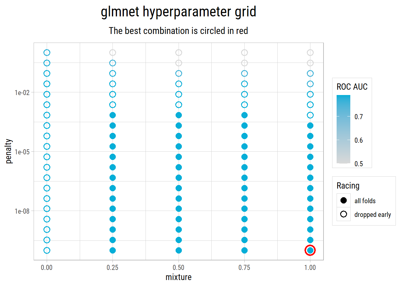

Non-linear Models

Next, we train two models that are built from decision trees. A decision tree splits the clients into groups with a series of yes/no questions, such as “Was the previous campaign a success?”. Tree models can learn curved relationships and interactions between features without our help.

ranger (Random Forest)

A random forest averages the predictions of many trees. Each tree learns from a random sample of the clients, and each split considers a random subset of the features. We use 500 trees and do a grid search of these hyperparameters:

mtry: The number of features to randomly sample at each split.
min_n: The minimum number of clients in a group required to split it further.

model_spec_rf

Random Forest Model Specification (classification)

Main Arguments:
  mtry = tune()
  trees = 500
  min_n = tune()

Engine-Specific Arguments:
  num.threads = 1

Computational engine: ranger

Let’s take a look at the top 10 hyperparameter combinations:

cv_results_rf %>% head(10)

# A tibble: 10 × 6
   min_n  mtry folds mn_log_loss pr_auc roc_auc
   <int> <int> <int>       <dbl>  <dbl>   <dbl>
 1    33     4     5       0.274  0.463   0.795
 2    15     3     5       0.274  0.461   0.795
 3    39     5     5       0.274  0.463   0.795
 4    22     3     5       0.275  0.461   0.794
 5    29     5     5       0.274  0.463   0.794
 6    33     7     5       0.275  0.462   0.794
 7    39     7     5       0.275  0.463   0.794
 8    18     6     5       0.276  0.461   0.793
 9    40     9     5       0.276  0.463   0.793
10     2     4     5       0.275  0.460   0.793

What’s notable?

The best ranger model has a ROC AUC of 0.795, with mtry = 4 and min_n = 33. It ranks clients better than the linear models.
Small values of mtry work best: the top 5 combinations sample only 3 to 5 features at each split. With few features to choose from, the trees are more different from each other, and their average is more reliable.
Racing dropped 11 of the 25 combinations after 3 folds.
ranger cross validation takes about 10 minutes.

cv_results_rf %>%
  mutate(racing = if_else(folds == max(folds), "all folds", "dropped early")) %>%
  ggplot(aes(x = min_n, y = mtry, color = roc_auc, shape = racing)) +
  geom_point(size = 3, stroke = 1) +
  geom_point(data = param_best_rf, aes(x = min_n, y = mtry), color = "red", size = 5, shape = 1, stroke = 1.5, inherit.aes = FALSE) +
  scale_color_gradient(low = "grey85", high = "#00AED8", name = "ROC AUC") +
  scale_shape_manual(values = c("all folds" = 16, "dropped early" = 1), name = "Racing") +
  scale_y_continuous(breaks = 1:10) +
  labs(title = "ranger hyperparameter grid", subtitle = "The best combination is circled in red")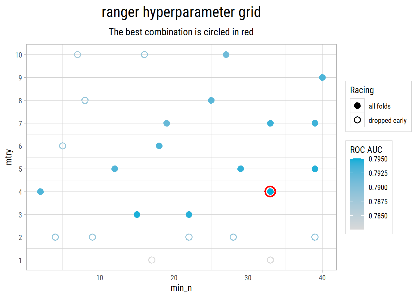

xgboost

Boosted trees add trees one at a time, and each new tree corrects the errors of the trees before it. We use 1,000 trees and do a grid search of these hyperparameters:

min_n: The minimum number of clients in a group required to split it further.
tree_depth: The maximum number of questions in a row in each tree.
learn_rate: How much each new tree changes the predictions.

model_spec_xgboost

Boosted Tree Model Specification (classification)

Main Arguments:
  trees = 1000
  min_n = tune()
  tree_depth = tune()
  learn_rate = tune()

Engine-Specific Arguments:
  nthread = 1

Computational engine: xgboost

Let’s take a look at the top 10 hyperparameter combinations:

cv_results_xgboost %>% head(10)

# A tibble: 10 × 7
   min_n tree_depth learn_rate folds mn_log_loss pr_auc roc_auc
   <int>      <int>      <dbl> <int>       <dbl>  <dbl>   <dbl>
 1    23          4    0.0254      5       0.274  0.460   0.800
 2    32          9    0.00605     5       0.273  0.461   0.799
 3     3          4    0.00418     5       0.274  0.462   0.799
 4    20          4    0.00401     5       0.275  0.457   0.798
 5    33          2    0.0289      5       0.275  0.457   0.797
 6     3          2    0.0171      5       0.275  0.457   0.797
 7    19         11    0.00482     5       0.274  0.461   0.797
 8    24          1    0.190       5       0.275  0.454   0.797
 9    29         15    0.00387     5       0.274  0.459   0.797
10     4          1    0.0872      4       0.276  0.457   0.797

What’s notable?

The best xgboost model has a ROC AUC of 0.800, with min_n = 23, tree_depth = 4 and learn_rate = 0.0254.
Racing dropped 16 of the 25 combinations after 3 folds. Of the 9 combinations that completed all the folds, 6 have shallow trees, with a depth of 4 or less. Small trees, added slowly, are enough for this data.
xgboost cross validation takes about 4 minutes.

Comparing the Models

dfCVSummary <- bind_rows(glm = cv_results_glm,
                         glmnet = cv_results_glmnet %>% slice(1),
                         ranger = cv_results_rf %>% slice(1),
                         xgboost = cv_results_xgboost %>% slice(1), .id = "model") %>%
  select(model, roc_auc, pr_auc, mn_log_loss) %>%
  left_join(dfTimings %>% mutate(seconds = round(seconds)), by = "model")

dfCVSummary %>%
  mutate(across(c(roc_auc, pr_auc, mn_log_loss), ~ round(.x, 4))) %>%
  knitr::kable(col.names = c("Model", "ROC AUC", "PR AUC", "Log loss", "Seconds to cross validate"))

Model	ROC AUC	PR AUC	Log loss	Seconds to cross validate
glm	0.7894	0.4462	0.2783	21
glmnet	0.7899	0.4454	0.2785	39
ranger	0.7950	0.4627	0.2741	613
xgboost	0.7997	0.4595	0.2738	266

What’s notable?

xgboost has the best ROC AUC, 0.800, and ranger has the best PR AUC, 0.463. The two tree models rank clients better than the two linear models, but only a little: the difference in ROC AUC is about 0.010.
So simple logistic regression gets most of the way. Most of the information is in a few strong features, which a linear model can use as well as a tree model.
The tree models take much longer to tune. ranger takes about 10 minutes, compared with 21 seconds for logistic regression.

Performance on Test Data

Now we use the final models to predict the probabilities of the 10,295 clients in the testing set, which the models have not seen.

get_test_probs <- function(model_final, label) {
  dfTest_Proc %>%
    select(Id, y) %>%
    mutate(model = label, .pred_yes = predict(model_final, dfTest_Proc, type = "prob")$.pred_yes)
}

dfTestPred <- bind_rows(get_test_probs(model_final_glm, "glm"),
                        get_test_probs(model_final_glmnet, "glmnet"),
                        get_test_probs(model_final_rf, "ranger"),
                        get_test_probs(model_final_xgboost, "xgboost"))

dfTestMetrics <- dfTestPred %>%
  group_by(model) %>%
  summarise(roc_auc = roc_auc_vec(y, .pred_yes),
            pr_auc = pr_auc_vec(y, .pred_yes),
            mn_log_loss = mn_log_loss_vec(y, .pred_yes))

dfTestMetrics %>%
  left_join(dfCVSummary %>% select(model, cv_roc_auc = roc_auc), by = "model") %>%
  mutate(across(where(is.numeric), ~ round(.x, 4))) %>%
  knitr::kable(col.names = c("Model", "Test ROC AUC", "Test PR AUC", "Test log loss", "Cross validated ROC AUC"))

Model	Test ROC AUC	Test PR AUC	Test log loss	Cross validated ROC AUC
glm	0.7957	0.4655	0.2746	0.7894
glmnet	0.7956	0.4643	0.2751	0.7899
ranger	0.8029	0.4780	0.2695	0.7950
xgboost	0.8027	0.4793	0.2691	0.7997

p1 <- dfTestPred %>%
  group_by(model) %>%
  roc_curve(y, .pred_yes) %>%
  ggplot(aes(x = 1 - specificity, y = sensitivity, color = model)) +
  geom_path(linewidth = 0.8) +
  geom_abline(lty = 2) +
  coord_equal() +
  scale_color_quant(palette = "metro") +
  labs(x = "False positive rate (1 - specificity)", y = "True positive rate (sensitivity)", title = "ROC curves")

p2 <- dfTestPred %>%
  group_by(model) %>%
  pr_curve(y, .pred_yes) %>%
  ggplot(aes(x = recall, y = precision, color = model)) +
  geom_path(linewidth = 0.8) +
  geom_hline(yintercept = mean(dfTest$y == "yes"), lty = 2) +
  coord_equal() +
  scale_color_quant(palette = "metro") +
  labs(x = "Recall", y = "Precision", title = "Precision-recall curves")

cowplot::plot_grid(plotlist = list(p1, p2), ncol = 2)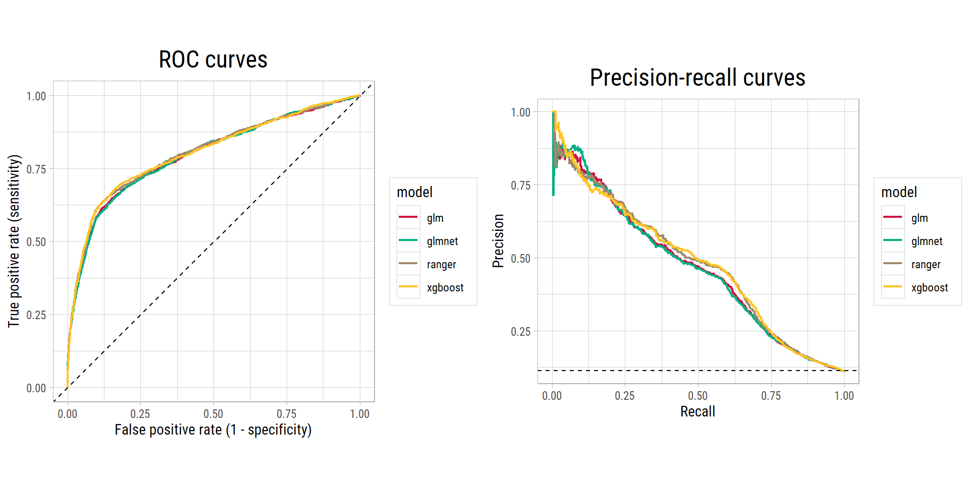

What’s notable?

On the testing set, each model does about as well as in cross validation, so the hyperparameters were not tuned to the training data by chance.
The tree models are again slightly better: ranger and xgboost have a test ROC AUC of 0.803 and 0.803, and logistic regression has 0.796.
A PR AUC of about 0.48 is about 4 times the 0.113 of a random ranking.
The ROC curves rise steeply at first: the clients with the highest probabilities are very likely to subscribe. After that, the models struggle to separate the remaining subscribers from the other clients.

How a Bank Could Use the Model

A bank cannot call every client. With a model, it can sort the clients by their predicted probability and call them from the top of the list. The gain curve shows the share of all the subscribers that the bank would reach, for each share of the clients that it calls:

dfTestPred %>%
  group_by(model) %>%
  gain_curve(y, .pred_yes) %>%
  ggplot(aes(x = .percent_tested / 100, y = .percent_found / 100, color = model)) +
  geom_path(linewidth = 0.8) +
  geom_abline(lty = 2) +
  scale_x_continuous(labels = scales::label_percent()) +
  scale_y_continuous(labels = scales::label_percent()) +
  scale_color_quant(palette = "metro") +
  labs(x = "Share of clients called (highest probability first)", y = "Share of subscribers reached",
       title = "Gain curves on the testing set", subtitle = "The dashed line is calling clients in random order")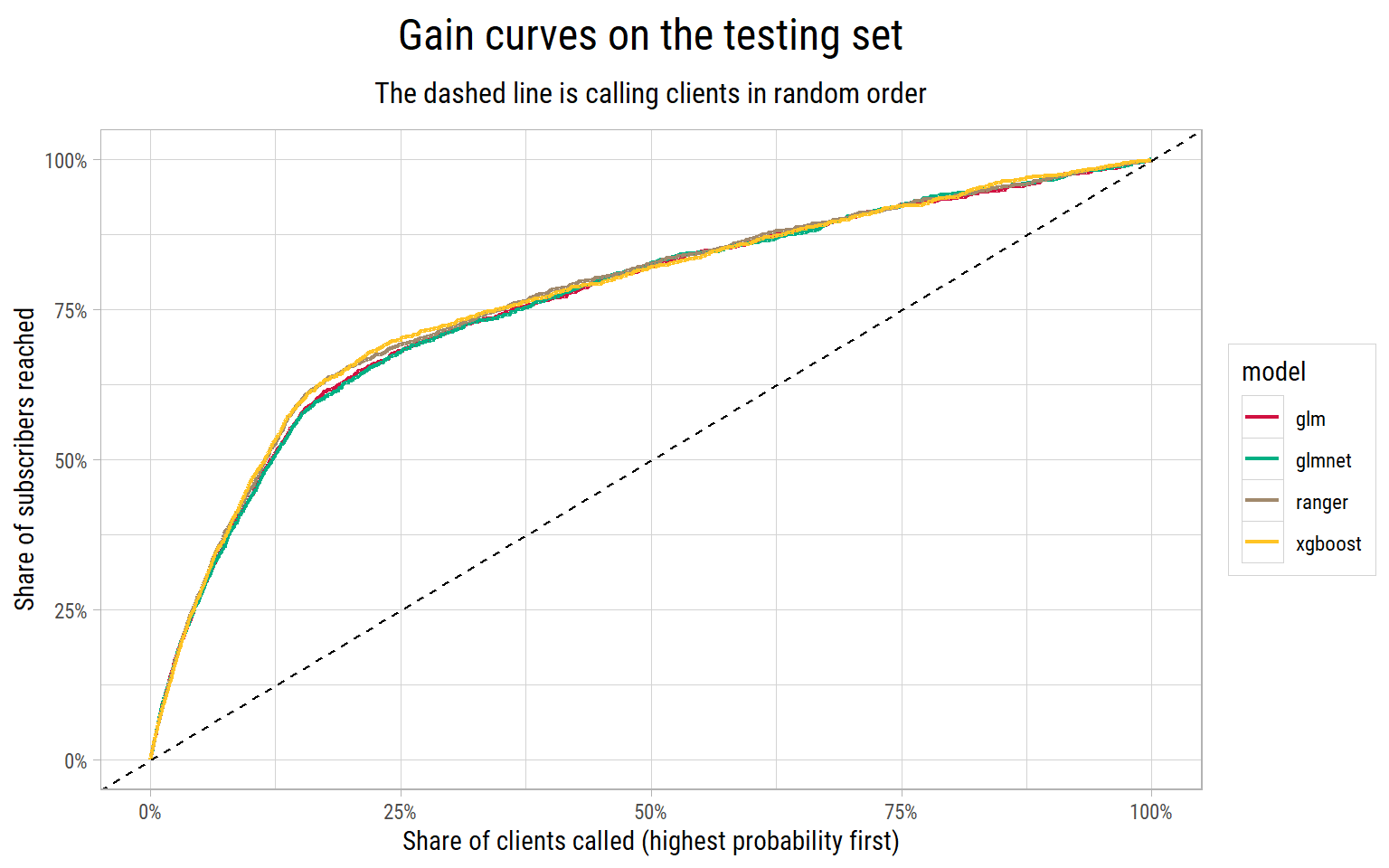

For the best model by cross validated ROC AUC, xgboost, here is what different call plans would achieve on the testing set:

dfBest <- dfTestPred %>% filter(model == best_model) %>% arrange(desc(.pred_yes))
overall_rate <- mean(dfBest$y == "yes")

dfCallPlans <- map_dfr(c(0.1, 0.2, 0.3, 0.5), function(share) {
  nCalled <- ceiling(share * nrow(dfBest))
  tibble(share_called = share,
         clients_called = nCalled,
         subscribers_reached = sum(dfBest$y[1:nCalled] == "yes") / sum(dfBest$y == "yes"),
         rate_among_called = mean(dfBest$y[1:nCalled] == "yes"),
         lift = rate_among_called / overall_rate)
})

dfCallPlans %>%
  mutate(across(c(share_called, subscribers_reached, rate_among_called), ~ scales::label_percent(accuracy = 1)(.x)),
         lift = round(lift, 1)) %>%
  knitr::kable(col.names = c("Share of clients called", "Clients called", "Share of subscribers reached",
                             "Subscription rate among clients called", "Lift"))

Share of clients called	Clients called	Share of subscribers reached	Subscription rate among clients called	Lift
10%	1030	47%	52%	4.7
20%	2059	66%	37%	3.3
30%	3089	73%	27%	2.4
50%	5148	82%	18%	1.6

The lift is the subscription rate among the clients called, divided by the overall rate of 11.3%.

What’s notable?

By calling the 10% of the clients with the highest probabilities, the bank would reach 47% of all the subscribers. 52% of these calls would end with a yes, 4.7 times the rate of calling at random.
Calling the top 20% reaches 66% of the subscribers. After that, each extra call finds fewer new subscribers: calling half of the clients reaches 82%.
The best plan depends on the cost of a call and on the value of a new deposit. The model gives the bank the list in the best order. The bank decides where to stop.

What Drives the Predictions?

The xgboost model is not as easy to read as a linear model, but it can tell us how much each feature improved its trees (the feature importance). The glmnet model is easier to read: for a categorical feature, the odds ratio of a category says how many times the odds of subscribing are multiplied for a client in that category, compared with the baseline category.

p1 <- vip::vip(extract_fit_parsnip(model_final_xgboost), num_features = 15, aesthetics = list(fill = "#00AED8")) +
  labs(title = "xgboost feature importance") +
  theme_quant()

# odds ratios of the categories (dummy variables) in the glmnet model. glmnet models the probability of the second
# level of y, which is "no", so the sign of each coefficient is reversed to give the odds of a "yes".
dfOddsRatios <- tidy(extract_fit_parsnip(model_final_glmnet)) %>%
  filter(str_detect(term, "_"), !term %in% vFeaturesEconomic, estimate != 0) %>%
  mutate(odds_ratio = exp(-estimate)) %>%
  slice_max(abs(estimate), n = 15) %>%
  mutate(term = fct_reorder(term, odds_ratio))

p2 <- ggplot(dfOddsRatios, aes(x = odds_ratio, y = term)) +
  geom_col(fill = "#F37735") +
  geom_vline(xintercept = 1, lty = 2) +
  scale_x_log10() +
  labs(x = "Odds ratio (log scale)", y = NULL, title = "glmnet: largest effects of categories")

cowplot::plot_grid(plotlist = list(p1, p2), ncol = 2)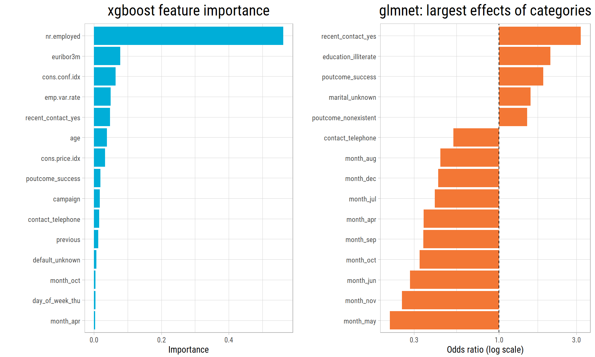

What’s notable?

In xgboost, nr.employed is by far the most important feature, and the other economic features follow. As we saw in Part 1, they tell the model when the call was made, and the subscription rate changed a lot over time.
Among the client features, the most important are the history with the bank (recent_contact, poutcome, previous), age, the number of calls in this campaign and the type of phone.
In glmnet, a recent contact in a previous campaign multiplies the odds of a yes by about 3.2, and a successful previous campaign by about 1.9 (compared with a failed one). A call to a landline about halves the odds.
Every month has lower odds than March, the baseline month, after taking the economy into account. March had the highest subscription rate in Part 1.
The large odds ratio of education_illiterate is not reliable, because only 18 clients have this category.

Testing on Later Calls

In Part 1, we saw that the economic features tell a model when a call was made, and that the subscription rate changed a lot over time. The testing set above has calls from the same period as the training set. But a bank would use the model to plan future calls.

So we train the best model (xgboost) again, with the same hyperparameters, on the first 75% of the calls in time order, and we test it on the last 25%. We do the same with logistic regression, the simplest model. We train each model twice: with all the features, and without the five economic features.

dfEarlyLateRates %>%
  mutate(rate = scales::label_percent(accuracy = 0.1)(rate)) %>%
  knitr::kable(col.names = c("Period", "Calls", "Subscription rate"))

Period	Calls	Subscription rate
earlier calls (training)	30882	6.4%
later calls (testing)	10294	25.8%

# the same earlier and later calls as in the tuning steps, where the best model was scored (dfLaterCalls)
dfAll_Proc <- bind_rows(dfTrain_Proc, dfTest_Proc) %>% arrange(Id)
idCutoff <- quantile(dfAll_Proc$Id, 0.75)
dfEarly_Proc <- dfAll_Proc %>% filter(Id <= idCutoff)
dfLate_Proc <- dfAll_Proc %>% filter(Id > idCutoff)

# logistic regression takes seconds to train, so it is scored here rather than in the tuning steps
score_glm_later_calls <- function(vExclude, features) {
  model_early <- workflow() %>%
    add_variables(outcomes = y, predictors = c(-Id, -any_of(vExclude))) %>%
    add_model(model_spec_glm) %>%
    fit(data = dfEarly_Proc)
  dfPred <- dfLate_Proc %>% select(y) %>% bind_cols(predict(model_early, dfLate_Proc, type = "prob"))
  tibble(features = features,
         roc_auc = roc_auc_vec(dfPred$y, dfPred$.pred_yes),
         pr_auc = pr_auc_vec(dfPred$y, dfPred$.pred_yes),
         mean_predicted = mean(dfPred$.pred_yes),
         actual_rate = mean(dfPred$y == "yes"))
}

dfLaterAll <- bind_rows(dfLaterCalls %>% mutate(model = best_model),
                        bind_rows(score_glm_later_calls(character(), "all features"),
                                  score_glm_later_calls(vFeaturesEconomic, "without economic features")) %>%
                          mutate(model = "glm")) %>%
  select(model, everything())

dfLaterAll %>%
  mutate(across(c(roc_auc, pr_auc), ~ round(.x, 3)),
         across(c(mean_predicted, actual_rate), ~ scales::label_percent(accuracy = 0.1)(.x))) %>%
  knitr::kable(col.names = c("Model", "Features", "ROC AUC on later calls", "PR AUC on later calls",
                             "Average predicted probability", "Actual subscription rate"))

Model	Features	ROC AUC on later calls	PR AUC on later calls	Average predicted probability	Actual subscription rate
xgboost	all features	0.611	0.342	20.8%	25.8%
xgboost	without economic features	0.503	0.308	18.1%	25.8%
glm	all features	0.275	0.164	8.2%	25.8%
glm	without economic features	0.707	0.469	18.1%	25.8%

later_value <- function(model, features, metric) dfLaterAll[[metric]][dfLaterAll$model == model & dfLaterAll$features == features]

# share of calls to clients whose previous campaign was a success, in each period
share_prev_success <- c(earlier = mean(dfEarly_Proc$poutcome_success == 1), later = mean(dfLate_Proc$poutcome_success == 1))

What’s notable?

The later calls are very different: 26% of them ended with a yes, compared with 6% of the earlier calls.
All the models do much worse on the later calls than on the random testing set. With all the features, xgboost has a ROC AUC of 0.611, compared with 0.803 on the random testing set. Without the economic features, its ROC AUC of 0.503 is no better than chance.
Logistic regression with all the features does even worse: its ROC AUC of 0.275 is below 0.5, so it ranks the clients in the wrong order. In the later calls, the economic features have values that the model never saw in training, such as interest rates below 1%. A linear model extends the straight-line trend that it learned, and here that trend points the wrong way.
Logistic regression without the economic features does best, with a ROC AUC of 0.707. In the earlier calls, only 0.4% of the clients had a successful previous campaign, compared with 12% in the later calls. The tree models saw too few of these clients to learn much from them, but logistic regression still learned one coefficient for them, and it carries over to the later calls.
So the random testing set gives a much too good picture of how the models would do in a future campaign. A bank should train the models again often, on its most recent calls, and test them on the calls that came after.

Conclusions

On calls from the same period, all the models rank the clients well, with a ROC AUC of about 0.8 on the testing set. The tree models are slightly better than logistic regression, but they take much longer to tune.
A bank could reach about 66% of the subscribers by calling only the top 20% of the clients on the list.
The strongest signals are the economy at the time of the call and the client’s history with the bank. The economic features make the models look good on a random testing set, but they do not carry over to a later period with a different economy.
When the data covers a period of time, a random testing set is not enough. We must also test the models on later data, which is how they will be used.

Appendix: Tuning Code

This is the code that tunes the models. It takes several minutes, so it does not run each time we build this page. Instead, the page saves the results in the file Bank_Tuning.Rda, together with a fingerprint (a hash) of the inputs of the tuning. The inputs are the clean data from Part 1 and the tuning code itself, which also sets the hyperparameter grids. When we build the page again, it calculates the fingerprint again:

If the fingerprint is the same, the page loads the saved results in a few seconds.
If the data, a hyperparameter or any other part of the tuning code has changed, the page tunes the models again and saves the new results.

Changes to the comments or the spacing of the code do not count as changes. To tune the models again without any change, delete Bank_Tuning.Rda.

These are the tuning steps:

# How the tuning code is built:
# It follows the tuning code of the Ames Housing case study (Part 3), adapted for classification:
#   1. The hyperparameters are tuned by racing (finetune::tune_race_anova), not by fitting every combination on every
#      fold: after 3 of the 5 folds, combinations that are clearly worse than the best are dropped (see "Cross
#      Validation Results"). Each (fold, combination) fit is a separate parallel task, so all workers stay busy.
#   2. The number of parallel workers is capped by available RAM as well as CPU cores (see "Parallel backend").
#   3. Models are compared by ROC AUC (see "Metrics"). Accuracy is not used: with 11% of clients subscribing, a model
#      that always predicts "no" is 89% accurate.
#   4. The models are logistic regression (the baseline, no hyperparameters), glmnet (regularized logistic regression),
#      ranger (random forest) and xgboost (boosted trees).
#      An SVM (kernlab), which the Ames case study also tuned, is not used here. Training an SVM takes time that grows
#      faster than the square of the number of rows, and each cross validation fit here has ~24,700 rows (17 times as
#      many as Ames). It also does not give class probabilities without an extra, slower calibration step.
#   5. After tuning, the best model is also trained on the earlier calls and tested on the later calls (see "Testing on
#      later calls"), because the economic features tell the model when a call was made (see Part 1). The post adds
#      logistic regression to this check outside the tuning steps, because it takes only seconds.
#
# Run time: the first version of this code fitted every combination on every fold, with mtry up to 20, a 25-point
# space-filling grid for glmnet and a 1 GB memory budget per worker (4 workers on this machine). A full run took ~28
# minutes: logistic regression 11s, glmnet 3 minutes, ranger 17 minutes and xgboost 6 minutes, plus the final fits.
# The changes in this version (racing, a regular grid for glmnet, mtry up to 10, 0.75 GB per worker) are explained
# where they are made. This version took ~17 minutes with 5 workers: logistic regression 21s (including starting the
# workers), glmnet 39s, ranger 10 minutes and xgboost 4.4 minutes, plus the final fits. Racing dropped 45 of the 100
# glmnet combinations, 11 of the 25 ranger combinations and 16 of the 25 xgboost combinations, and it kept the same
# best xgboost combination. The saving is less than the share of dropped combinations, because every combination is
# fitted on 3 of the 5 folds before any is dropped. All R processes together peaked at 4.9 GB.

# load the clean dataset from Part 1 (bank_data_file is set in the "tuning_cache" chunk)
load(bank_data_file)

# Training and testing sets (the stratified split was made in Part 1)
########################################################################################################################################################
dfTrain <- dfClean %>% filter(!(Id %in% vTestIDs))
dfTest <- dfClean %>% filter(Id %in% vTestIDs)

# Right-skewed numerical features (a long tail of large values), which are log transformed for the linear models
# (tree models are not affected by it). Only positive skewness counts: nr.employed is skewed to the left, and the log
# of an employment count would not make its distribution more even.
vFeaturesSkew <- dfClean %>%
    select(all_of(vFeaturesNum)) %>%
    select_if(function(Z) timeDate::skewness(Z, na.rm = T) > 0.75) %>%
    colnames()

# Preprocessing Recipe
########################################################################################################################################################
# Categorical features become dummy variables (one 0/1 predictor per category but one). The "unknown" categories of
# housing and loan are the same 990 clients, so those two dummy variables are identical. step_lincomb removes exact
# linear combinations like this one. An intercept column is added for the check, because such combinations can include
# a constant, and removed afterwards. step_zv removes predictors with a single value.
get_preprocessing_recipe <- function(df) {

    recipe(y ~ ., data = df) %>%
        update_role(Id, new_role = "ID") %>%
        step_mutate_at(all_of(vFeaturesSkew), fn = ~ log(. + 1)) %>%
        step_dummy(all_nominal_predictors()) %>%
        step_zv(all_predictors()) %>%
        step_intercept() %>%
        step_lincomb(all_numeric_predictors()) %>%
        step_rm(any_of("intercept")) %>%
        prep()
}

# The recipe is prepared on the training set only, and the same recipe is applied to the testing set (and to any new
# data), so that both have exactly the same predictors.
preprocessing_recipe <- get_preprocessing_recipe(dfTrain)
dfTrain_Proc <- preprocessing_recipe %>% bake(new_data = NULL)
dfTest_Proc <- preprocessing_recipe %>% bake(new_data = dfTest)


# Metrics
########################################################################################################################################################
# ROC AUC: the probability that a random subscriber gets a higher predicted probability than a random non-subscriber.
#          It measures how well the model ranks clients, which is what a bank needs to decide whom to call first.
# PR AUC:  the average precision (share of subscribers among the clients called) over all recall levels. It focuses on
#          the rare class, so it shows differences between models that ROC AUC can hide when classes are imbalanced.
# Log loss: measures how good the probabilities themselves are (lower is better).
# "yes" is the first level of y, so it is the event for all three metrics.
class_metrics <- metric_set(roc_auc, pr_auc, mn_log_loss)


# Parsnip Model Specification
########################################################################################################################################################
get_model_spec <- function(modelType) {

    model_spec <- switch(modelType,
                         glm = logistic_reg(mode = "classification") %>%
                             set_engine("glm"),

                         glmnet = logistic_reg(mode = "classification", penalty = tune(), mixture = tune()) %>%
                             set_engine("glmnet"),

                         # 500 trees, as in the Ames case study: random forest performance levels off well before that.
                         # num.threads = 1 because parallelism comes from running many fits at once (one per worker).
                         ranger = rand_forest(mode = "classification", trees = 500, mtry = tune(), min_n = tune()) %>%
                             set_engine("ranger", num.threads = 1),

                         # No early stopping, for the reason found in the Ames case study: with a random validation split,
                         # the stopping point, and so the final model, changed from one run to the next.
                         xgboost = boost_tree(mode = "classification", trees = 1000, min_n = tune(), tree_depth = tune(),
                                              learn_rate = tune()) %>%
                             set_engine("xgboost", nthread = 1))

    return(model_spec)
}


# Parameter Grid Search
########################################################################################################################################################
get_model_param_grid <- function(df, modelType, numParams, randomSeed) {

    # glmnet gets a regular grid: 20 penalties for each of 5 mixtures. glmnet calculates the coefficients for a whole
    # sequence of penalties in one fit, and tune uses this when the grid has several penalties for the same mixture
    # (penalty is a "submodel" parameter). So 100 combinations need only 5 fits per fold, while the 25-point
    # space-filling grid, with a different mixture in every point, needed 25.
    if(modelType == "glmnet") {
        return(grid_regular(penalty(), mixture(), levels = c(penalty = 20, mixture = 5)))
    }

    set.seed(randomSeed)
    param_spec <- switch(modelType,
                         # learn_rate is on a log10 scale; ~0.003 to ~0.3 covers the useful range for 1,000 trees (see the
                         # Ames case study, where the dials default spent most of the grid on rates that never converged).
                         xgboost = parameters(min_n(), tree_depth(), learn_rate(range = c(-2.5, -0.5))),
                         # mtry is limited to 1-10 of the ~50 predictors. Small values win, and the time of a fit grows with
                         # mtry. In a test run over the full range, mtry 6 and 2 had ROC AUC 0.794 and 0.793, and mtry 35-37
                         # had 0.781-0.788. On one fold, with 500 trees and min_n = 10: mtry 6 took 14.4s (ROC AUC 0.788),
                         # mtry 20 took 30.7s (0.784) and mtry 35 took 46.2s (0.780). In a full run with mtry up to 20, all
                         # 5 best combinations had mtry 2 to 7, and ranger still took 62% of the tuning time.
                         ranger = parameters(min_n(), mtry(range = c(1, 10))))

    dfParamGrid <- grid_space_filling(param_spec, size = numParams, type = "max_entropy")
    return(dfParamGrid)
}


# Workflow for a model
########################################################################################################################################################
# The data is already preprocessed, so the workflow only names the outcome and predictors.
# Id is excluded from the predictors: it is the order of the calls, so a tree model could otherwise split on it and
# learn the period of a call directly. vExclude removes more predictors (used in "Testing on later calls").
get_workflow <- function(model_spec, vExclude = character()) {
    workflow() %>%
        add_variables(outcomes = y, predictors = c(-Id, -any_of(vExclude))) %>%
        add_model(model_spec)
}


# Cross Validation Results
########################################################################################################################################################
# Racing (finetune::tune_race_anova): every combination is first fitted on 3 folds (the burn-in). Then a statistical
# test (ANOVA) on the ROC AUC, the first metric in class_metrics, drops the combinations that are clearly worse than the
# best one, and only the remaining combinations are fitted on the next fold, and so on. With parallel_over =
# "everything", each (fold, combination) fit is a separate task, so all workers stay busy.
# The results have one row per combination, with the mean of each metric over the folds that it completed. The
# combinations that completed all the folds come first, best ROC AUC first; the dropped ones follow.
cross_validate_model <- function(cv_folds, model_spec, param_grid) {

    tune_results <- get_workflow(model_spec) %>%
        finetune::tune_race_anova(resamples = cv_folds,
                                  grid = param_grid,
                                  metrics = class_metrics,
                                  control = finetune::control_race(burn_in = 3, parallel_over = "everything"))

    # all_configs = TRUE keeps the dropped combinations, which collect_metrics() leaves out of race results by default
    dfResults <- tune_results %>%
        collect_metrics(all_configs = TRUE) %>%
        select(all_of(names(param_grid)), .metric, mean, folds = n) %>%
        pivot_wider(names_from = .metric, values_from = mean) %>%
        arrange(desc(folds), desc(roc_auc))
    return(dfResults)
}


# Fitted model with parameters
########################################################################################################################################################
# Returns a fitted workflow; predict() on it selects the predictor columns from new data, so Id can stay in the data.
# The seed makes the final ranger and xgboost fits reproducible between runs.
get_fitted_model <- function(df, model_spec, dfParams, randomSeed = 2300, vExclude = character()) {

    model_wf <- get_workflow(model_spec, vExclude)
    if(!is.null(dfParams)) model_wf <- model_wf %>% finalize_workflow(dfParams)
    set.seed(randomSeed)
    fit(model_wf, data = df)
}


# Parallel backend
########################################################################################################################################################
# Each worker is a separate R session with tidymodels and the model packages loaded. The training set here is 21 times
# the size of the Ames training set, and one ranger probability forest of 500 trees takes ~150 MB. In a full run with
# 4 workers, all R processes together peaked at 3.4 GB, of which the main session (which holds the data and the final
# models) used 1.1 GB, so each worker used ~0.6 GB. Budgeting 0.75 GB per worker leaves headroom. Workers are capped
# at cores - 1 (to keep the machine responsive) and at what fits in 70% of the RAM available when the run starts, so
# the run cannot push the machine into swapping. On a CPU with 4 cores and 8 threads (hyperthreading), workers beyond
# 4 share cores, so they add less than a full core each.
gb_per_worker <- 0.75
gb_available <- ps::ps_system_memory()$avail / 1024^3
num_workers <- max(1, min(parallel::detectCores() - 1, floor(0.7 * gb_available / gb_per_worker)))
message(sprintf("Using %d parallel workers (%.1f GB RAM available)", num_workers, gb_available))
plan(multisession, workers = num_workers)

# Create cross validation folds, stratified so that each fold has the same subscription rate
set.seed(2300)
cv_folds <- vfold_cv(dfTrain_Proc, v = 5, strata = y)

# Time each model so the post can report relative run times
dfTimings <- tibble(model = character(), seconds = numeric())
time_model <- function(model, expr) {
    t0 <- Sys.time()
    result <- force(expr)
    dfTimings <<- dfTimings %>% add_row(model = model, seconds = as.numeric(difftime(Sys.time(), t0, units = "secs")))
    result
}

# logistic regression (no hyperparameters, so fit_resamples instead of tune_grid)
model_spec_glm <- get_model_spec(modelType = "glm")
cv_results_glm <- time_model("glm",
    get_workflow(model_spec_glm) %>%
        fit_resamples(resamples = cv_folds, metrics = class_metrics) %>%
        collect_metrics() %>%
        select(.metric, mean) %>%
        pivot_wider(names_from = .metric, values_from = mean))
model_final_glm <- get_fitted_model(dfTrain_Proc, model_spec_glm, NULL)

# glmnet model
model_spec_glmnet <- get_model_spec(modelType = "glmnet")
param_grid_glmnet <- get_model_param_grid(dfTrain_Proc, modelType = "glmnet", numParams = 25, randomSeed = 2300)
cv_results_glmnet <- time_model("glmnet", cross_validate_model(cv_folds, model_spec_glmnet, param_grid_glmnet))
param_best_glmnet <- cv_results_glmnet %>% slice(1) %>% select(all_of(names(param_grid_glmnet)))
model_final_glmnet <- get_fitted_model(dfTrain_Proc, model_spec_glmnet, param_best_glmnet)

# random forest model (ranger engine)
model_spec_rf <- get_model_spec(modelType = "ranger")
param_grid_rf <- get_model_param_grid(dfTrain_Proc, modelType = "ranger", numParams = 25, randomSeed = 2300)
cv_results_rf <- time_model("ranger", cross_validate_model(cv_folds, model_spec_rf, param_grid_rf))
param_best_rf <- cv_results_rf %>% slice(1) %>% select(all_of(names(param_grid_rf)))
model_final_rf <- get_fitted_model(dfTrain_Proc, model_spec_rf, param_best_rf)

# xgboost model
model_spec_xgboost <- get_model_spec(modelType = "xgboost")
param_grid_xgboost <- get_model_param_grid(dfTrain_Proc, modelType = "xgboost", numParams = 25, randomSeed = 2300)
cv_results_xgboost <- time_model("xgboost", cross_validate_model(cv_folds, model_spec_xgboost, param_grid_xgboost))
param_best_xgboost <- cv_results_xgboost %>% slice(1) %>% select(all_of(names(param_grid_xgboost)))
model_final_xgboost <- get_fitted_model(dfTrain_Proc, model_spec_xgboost, param_best_xgboost)

plan(sequential)


# Testing on later calls
########################################################################################################################################################
# The random split above tests the models on calls from the same period as the training calls. Here, the best model
# by cross validated ROC AUC is trained on the first 75% of the calls (in time order, Id) and tested on the last 25%,
# with the same hyperparameters, once with all the features and once without the five economic features.
vFeaturesEconomic <- c("emp.var.rate", "cons.price.idx", "cons.conf.idx", "euribor3m", "nr.employed")
dfAll_Proc <- bind_rows(dfTrain_Proc, dfTest_Proc) %>% arrange(Id)
idCutoff <- quantile(dfAll_Proc$Id, 0.75)
dfEarly_Proc <- dfAll_Proc %>% filter(Id <= idCutoff)
dfLate_Proc <- dfAll_Proc %>% filter(Id > idCutoff)

dfCVBest <- bind_rows(glmnet = cv_results_glmnet %>% slice(1), ranger = cv_results_rf %>% slice(1),
                      xgboost = cv_results_xgboost %>% slice(1), .id = "model")
best_model <- dfCVBest$model[which.max(dfCVBest$roc_auc)]
best_spec <- switch(best_model, glmnet = model_spec_glmnet, ranger = model_spec_rf, xgboost = model_spec_xgboost)
best_params <- switch(best_model, glmnet = param_best_glmnet, ranger = param_best_rf, xgboost = param_best_xgboost)

score_later_calls <- function(vExclude, features) {
    model_early <- get_fitted_model(dfEarly_Proc, best_spec, best_params, vExclude = vExclude)
    dfPred <- dfLate_Proc %>% select(y) %>% bind_cols(predict(model_early, dfLate_Proc, type = "prob"))
    tibble(features = features,
           roc_auc = roc_auc_vec(dfPred$y, dfPred$.pred_yes),
           pr_auc = pr_auc_vec(dfPred$y, dfPred$.pred_yes),
           mean_predicted = mean(dfPred$.pred_yes),
           actual_rate = mean(dfPred$y == "yes"))
}
dfLaterCalls <- bind_rows(score_later_calls(character(), "all features"),
                          score_later_calls(vFeaturesEconomic, "without economic features"))
dfEarlyLateRates <- tibble(period = c("earlier calls (training)", "later calls (testing)"),
                           calls = c(nrow(dfEarly_Proc), nrow(dfLate_Proc)),
                           rate = c(mean(dfEarly_Proc$y == "yes"), mean(dfLate_Proc$y == "yes")))


# the results that the post uses, which are saved to Bank_Tuning.Rda
vTuningResults <- c("model_spec_glm", "model_spec_glmnet", "model_spec_rf", "model_spec_xgboost",
                    "model_final_glm", "model_final_glmnet", "model_final_rf", "model_final_xgboost",
                    "cv_results_glm", "cv_results_glmnet", "cv_results_rf", "cv_results_xgboost",
                    "param_grid_glmnet", "param_grid_rf", "param_grid_xgboost",
                    "param_best_glmnet", "param_best_rf", "param_best_xgboost",
                    "dfTrain", "dfTest", "dfTrain_Proc", "dfTest_Proc", "preprocessing_recipe", "vFeaturesSkew",
                    "cv_folds", "dfTimings", "num_workers", "best_model", "dfLaterCalls", "dfEarlyLateRates",
                    "vFeaturesEconomic")

And this code decides whether to load the saved results or to run the tuning steps:

# The clean dataset from Part 1
bank_data_file <- "../bank-marketing-part1-eda/Bank_Marketing_Clean.Rda"

# Fingerprint (hash) of the inputs of the tuning: the data that it uses, and the code of the "tuning_steps"
# chunk, which also sets the hyperparameter grids. Comments and spacing are removed from the code first, so
# editing them does not start a new tuning run.
envData <- new.env()
load(bank_data_file, envir = envData)
tuning_steps <- knitr::knit_code$get("tuning_steps")
tuning_hash <- rlang::hash(list(data = list(envData$dfClean, envData$vTestIDs),
                                code = deparse(parse(text = tuning_steps, keep.source = FALSE))))

# If the saved results were made from the same inputs, load them. Otherwise, tune the models again and save
# the new results together with the fingerprint of their inputs.
envSaved <- new.env()
if (file.exists("Bank_Tuning.Rda")) load("Bank_Tuning.Rda", envir = envSaved)
if (identical(envSaved$tuning_hash, tuning_hash)) {
  list2env(as.list(envSaved), envir = environment())
} else {
  eval(parse(text = tuning_steps))
  save(list = c(vTuningResults, "tuning_hash"), file = "Bank_Tuning.Rda")
}
rm(envData, envSaved)

rstats ggplot2 models classification logistic regression glmnet ranger xgboost

Bank Marketing - Part 2 - Who will say yes? - Building Classification Models

Other posts in this series:

Evaluation Criteria

Steps for Building Models

Preparing the Features

Partitioning Training Data

Linear Models

Logistic Regression

What’s notable?

Regularized Logistic Regression

What’s notable?

Non-linear Models

ranger (Random Forest)

What’s notable?

xgboost

What’s notable?

Comparing the Models

What’s notable?

Performance on Test Data

What’s notable?

How a Bank Could Use the Model

What’s notable?

What Drives the Predictions?

What’s notable?

Testing on Later Calls

What’s notable?

Conclusions

Appendix: Tuning Code

Related