Bank Marketing - Part 1 - Making the call - An Exploratory Data Analysis
Other posts in this series:
A Portuguese bank ran a series of telemarketing campaigns between May 2008 and November 2010. Its staff called clients and asked them to open a term deposit, a savings account that pays a fixed interest rate for a fixed period. The Bank Marketing dataset (Moro, Cortez and Rita, 2014) records 41,188 of these calls: who the client was, how and when they were called, the state of the economy at the time, and whether the client said yes.
In the Ames Housing and Diamonds case studies, we predicted a number (a price). Here, we predict a category: will a client subscribe, yes or no? This kind of problem is called classification. The case study has two posts:
- In this post, we explore the data to find which features affect whether a client subscribes, and we prepare the data for models. An exploratory data analysis (EDA) is the first study of a dataset before we build models.
- In Part 2, we build models that predict which clients will subscribe, and we find out how a bank could use them to decide whom to call.
Data Description
Each row is one call, which was the last call to a client in a campaign. The rows are in the order of the calls, from May 2008 to November 2010. There are 20 features and the target, y, which is the value that we want to predict:
dfDescription <- tribble(~ Feature, ~ Type, ~ Description,
                         "age", "numerical", "age of the client",
                         "job", "categorical", "type of job",
                         "marital", "categorical", "marital status (*divorced* also means widowed)",
                         "education", "categorical", "highest level of education",
                         "default", "categorical", "does the client have a loan in default?",
                         "housing", "categorical", "does the client have a housing loan?",
                         "loan", "categorical", "does the client have a personal loan?",
                         "contact", "categorical", "type of phone: cellular or telephone (landline)",
                         "month", "categorical", "month of the call",
                         "day_of_week", "categorical", "day of the week of the call",
                         "duration", "numerical", "length of the call, in seconds",
                         "campaign", "numerical", "number of calls to the client in this campaign, including this one",
                         "pdays", "numerical", "days since the client was last called in a previous campaign (999: not called)",
                         "previous", "numerical", "number of calls to the client before this campaign",
                         "poutcome", "categorical", "result of the previous campaign",
                         "emp.var.rate", "numerical", "employment variation rate (quarterly)",
                         "cons.price.idx", "numerical", "consumer price index (monthly)",
                         "cons.conf.idx", "numerical", "consumer confidence index (monthly)",
                         "euribor3m", "numerical", "3 month Euribor interest rate (daily)",
                         "nr.employed", "numerical", "number of employees in the economy, in thousands (quarterly)",
                         "y", "categorical", "**target**: did the client subscribe to a term deposit?")

knitr::kable(dfDescription)| Feature | Type | Description |
|---|---|---|
| age | numerical | age of the client |
| job | categorical | type of job |
| marital | categorical | marital status (divorced also means widowed) |
| education | categorical | highest level of education |
| default | categorical | does the client have a loan in default? |
| housing | categorical | does the client have a housing loan? |
| loan | categorical | does the client have a personal loan? |
| contact | categorical | type of phone: cellular or telephone (landline) |
| month | categorical | month of the call |
| day_of_week | categorical | day of the week of the call |
| duration | numerical | length of the call, in seconds |
| campaign | numerical | number of calls to the client in this campaign, including this one |
| pdays | numerical | days since the client was last called in a previous campaign (999: not called) |
| previous | numerical | number of calls to the client before this campaign |
| poutcome | categorical | result of the previous campaign |
| emp.var.rate | numerical | employment variation rate (quarterly) |
| cons.price.idx | numerical | consumer price index (monthly) |
| cons.conf.idx | numerical | consumer confidence index (monthly) |
| euribor3m | numerical | 3 month Euribor interest rate (daily) |
| nr.employed | numerical | number of employees in the economy, in thousands (quarterly) |
| y | categorical | target: did the client subscribe to a term deposit? |
The last five features describe the economy of Portugal at the time of the call. They are the same for all the clients who were called on the same day.
Data Quality
Before we explore the features, we check the data for problems.
# exact duplicate rows
nDuplicates <- sum(duplicated(dfRaw))

# number of "unknown" values in each categorical feature
dfUnknown <- dfRaw %>%
  select(where(is.character)) %>%
  summarise(across(everything(), ~ sum(.x == "unknown"))) %>%
  pivot_longer(everything(), names_to = "feature", values_to = "unknown") %>%
  filter(unknown > 0) %>%
  mutate(percent = round(100 * unknown / nrow(dfRaw), 1)) %>%
  arrange(desc(unknown))

knitr::kable(dfUnknown, col.names = c("Feature", "Unknown values", "% of calls"))| Feature | Unknown values | % of calls |
|---|---|---|
| default | 8597 | 20.9 |
| education | 1731 | 4.2 |
| housing | 990 | 2.4 |
| loan | 990 | 2.4 |
| job | 330 | 0.8 |
| marital | 80 | 0.2 |
# clients called in a previous campaign, by whether pdays is recorded
dfPrevious <- dfRaw %>%
  filter(previous > 0) %>%
  count(pdays_recorded = pdays != 999, poutcome)
What’s notable?
- There are no empty (missing) values. Instead, the categorical features use the category unknown.
defaultis unknown for 20.9% of the clients.housingandloanare unknown for the same 990 clients. - 12 rows are exact copies of other rows. The data has no client ID, so we cannot tell whether these are the same call recorded twice or different clients with the same details. They are too few to matter, and we remove them when we prepare the data.
defaulthas only 3 clients with yes. So the feature really tells us whether the client’s answer was no or unknown.- The description says that a
pdaysof 999 means the client was not called before. But 5,625 clients were called in a previous campaign (previousis more than 0), and only 1,515 of them have apdaysvalue. Of those, 1373 had a successful previous campaign. Sopdaysis mostly recorded for clients who said yes before.
The Target: Who Subscribed?
dfTarget <- dfRaw %>% count(y) %>% mutate(percent = 100 * n / sum(n))
rate_yes <- mean(dfRaw$y == "yes")

ggplot(dfTarget, aes(x = y, y = n, fill = y)) +
  geom_col(show.legend = FALSE) +
  geom_text(aes(label = glue::glue("{format(n, big.mark = ',')} ({round(percent, 1)}%)")), vjust = -0.5, family = "Roboto Condensed") +
  scale_fill_quant(palette = "main") +
  scale_y_continuous(labels = scales::label_comma(), expand = expansion(mult = c(0, 0.1))) +
  labs(x = "Subscribed to a term deposit (y)", y = "Number of calls", title = "Most clients said no")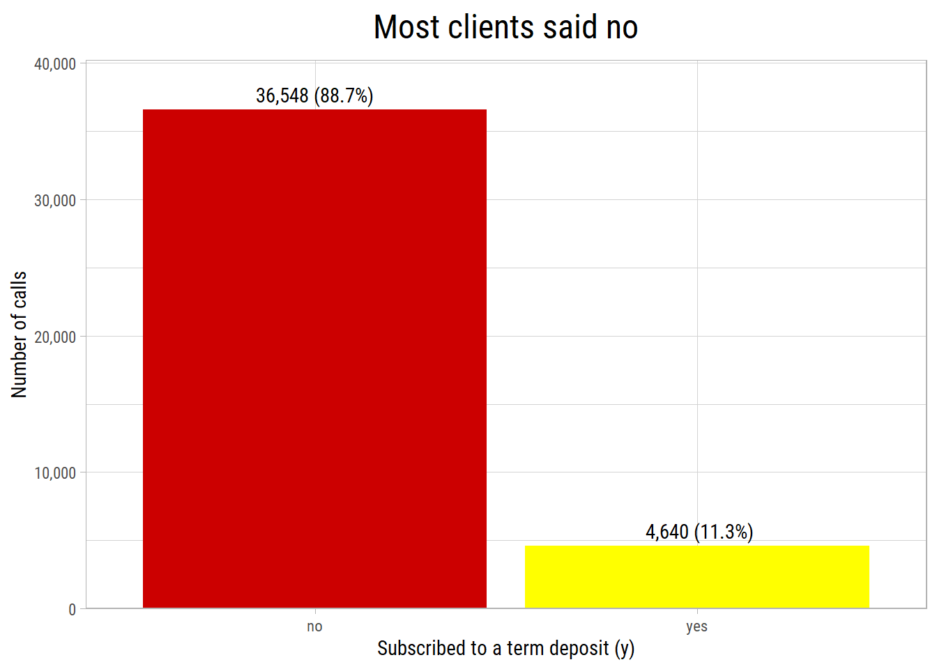
What’s notable?
- Only 11.3% of the calls ended with a subscription. The two classes are very unequal in size (imbalanced).
- So a model that always predicts no would be right 88.7% of the time, but it would be useless. In Part 2, we use measures that are not fooled by this.
In the rest of this post, we compare the subscription rate, the percentage of calls that ended with a yes, across the values of each feature. The dashed line in the plots is the overall rate of 11.3%. These functions make the plots:
# subscription rate and number of calls for each category of a feature
plot_rate <- function(df, feature, sortByRate = TRUE, minCount = 30) {
  dfRate <- df %>%
    group_by(category = .data[[feature]]) %>%
    summarise(calls = n(), rate = mean(y == "yes"), .groups = "drop") %>%
    filter(calls >= minCount)
  if (sortByRate) dfRate <- dfRate %>% mutate(category = fct_reorder(as.factor(category), rate))
  ggplot(dfRate, aes(x = category, y = rate)) +
    geom_col(fill = "#00AED8") +
    geom_hline(yintercept = mean(df$y == "yes"), lty = 2) +
    geom_text(aes(label = scales::label_comma()(calls)), hjust = -0.1, size = 3, family = "Roboto Condensed") +
    scale_y_continuous(labels = scales::label_percent(), expand = expansion(mult = c(0, 0.25))) +
    coord_flip() +
    labs(x = NULL, y = "Subscription rate", title = feature)
}

# subscription rate for bins of a numerical feature
plot_rate_bins <- function(df, feature, breaks, labels = NULL) {
  df %>%
    mutate(bin = cut(.data[[feature]], breaks = breaks, labels = labels, include.lowest = TRUE, dig.lab = 5)) %>%
    plot_rate("bin", sortByRate = FALSE) +
    labs(title = feature)
}
The numbers next to the bars are the numbers of calls. Categories with fewer than 30 calls are not shown, because their rates are not reliable.
A Feature We Cannot Use: Call Duration
plot_rate_bins(dfRaw, "duration", breaks = c(0, 60, 120, 180, 300, 600, 5000)) +
  labs(x = "Length of the call (seconds)")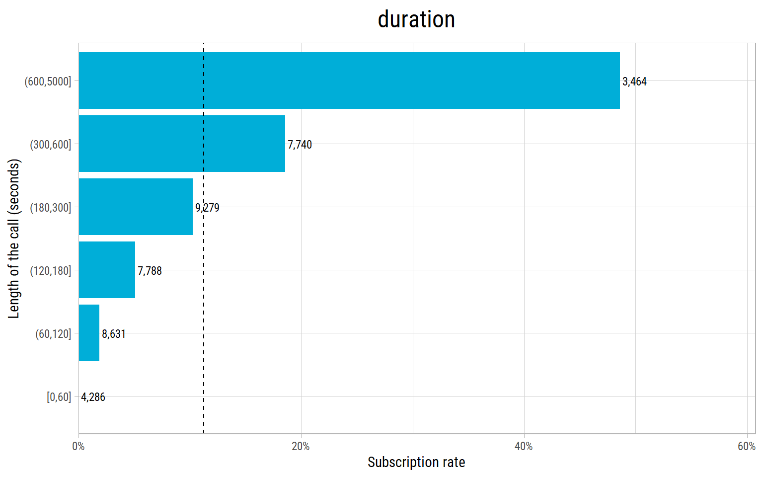
What’s notable?
durationpredicts the result very well: almost no client who talked for less than a minute subscribed, and about half of the clients who talked for more than 10 minutes did.- But we only know the length of a call after the call has ended, and by then we also know whether the client said yes. A bank cannot use it to decide whom to call. Using a feature that would not be known at the time of the prediction is called data leakage. It makes a model look much better than it will be in practice.
- The authors of the dataset give the same warning. So we drop
duration.
Univariate Analysis: One Feature at a Time
Numerical Features
vFeaturesNumRaw <- c("age", "campaign", "previous", "emp.var.rate", "cons.price.idx", "cons.conf.idx", "euribor3m", "nr.employed")
eda_plot_histograms(dfRaw, vFeaturesNumRaw, nCols = 4)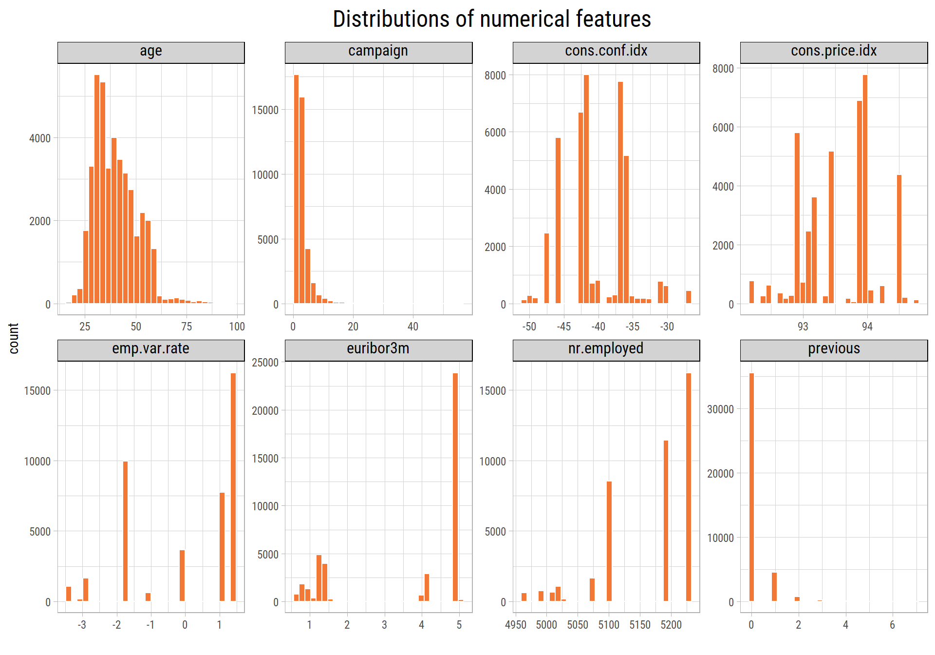
What’s notable?
- Most clients are between 30 and 50 years old.
- Most clients were called once or twice in the campaign, but some were called up to 56 times.
campaignis very skewed. - Most clients (86%) were never called in a previous campaign.
- The economic features have only a few distinct values, with gaps between them. For example,
nr.employedhas only 11 values, because it changes once a quarter. So these features also tell us when a call was made.
Categorical Features
vFeaturesCatRaw <- c("job", "marital", "education", "default", "housing", "loan", "contact", "month", "day_of_week", "poutcome")
cowplot::plot_grid(plotlist = map(vFeaturesCatRaw, ~ eda_plot_column(dfRaw, .x)), ncol = 3)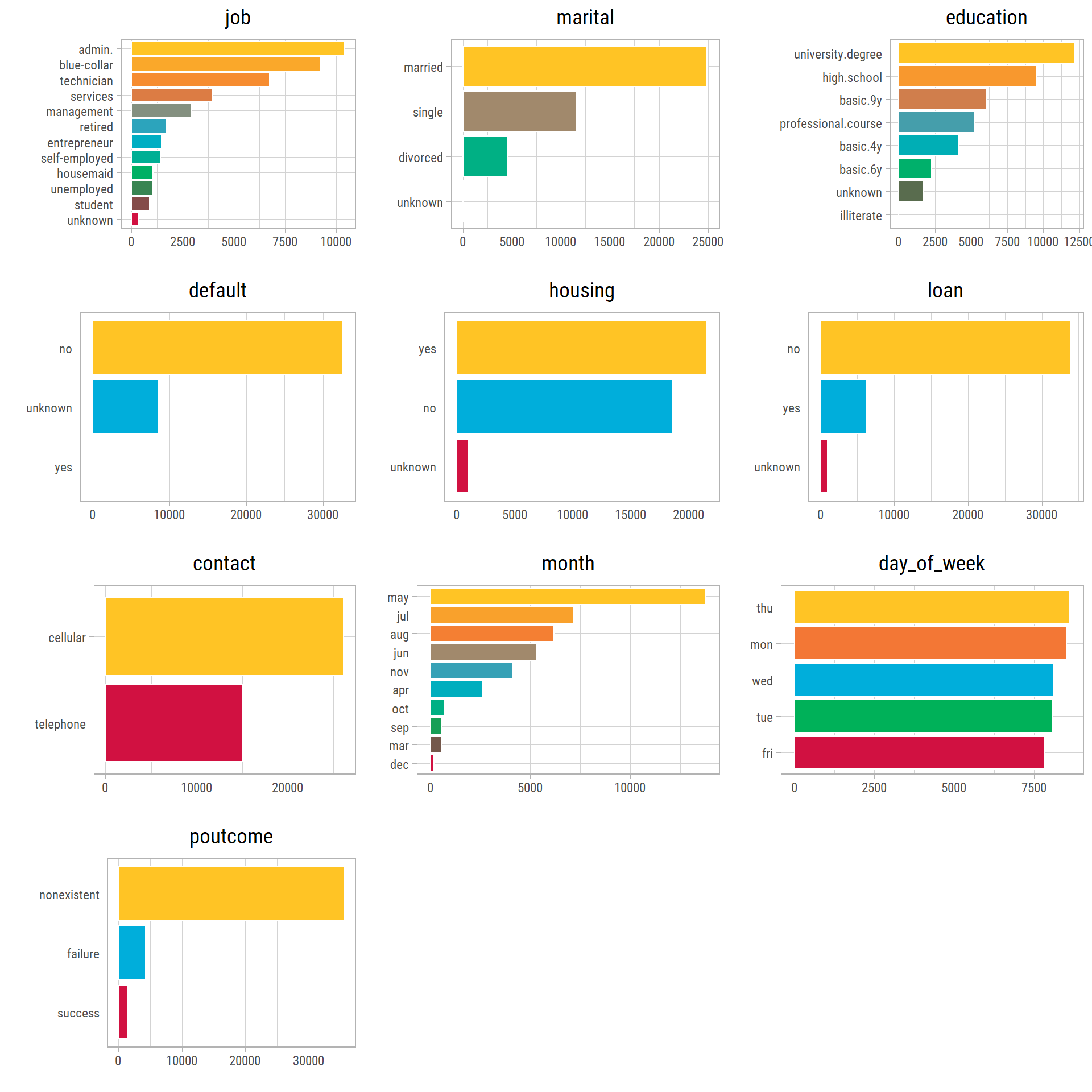
What’s notable?
- Most clients work in administration, blue-collar jobs or as technicians.
- Most calls were made in May, and the fewest in December and March. There are no calls in January and February.
- About two thirds of the calls were to cell phones.
Bivariate Analysis: Each Feature and the Subscription Rate
Client Features
p1 <- plot_rate_bins(dfRaw, "age", breaks = c(17, 25, 30, 40, 50, 60, 100))
p2 <- plot_rate(dfRaw, "job")
p3 <- plot_rate(dfRaw, "marital")
p4 <- plot_rate(dfRaw, "education")
p5 <- plot_rate(dfRaw, "default")
p6 <- plot_rate(dfRaw, "housing")
cowplot::plot_grid(plotlist = list(p1, p2, p3, p4, p5, p6), ncol = 2)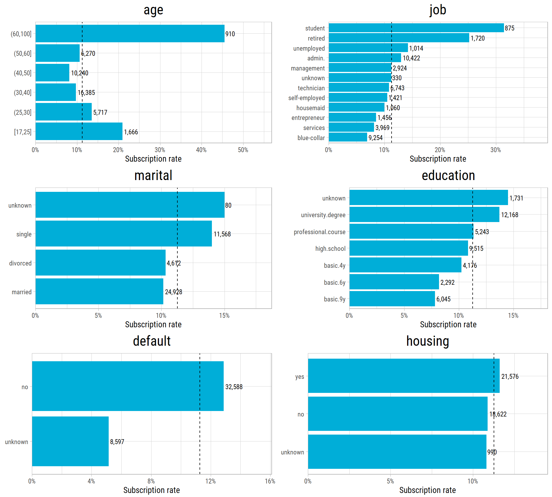
What’s notable?
- The youngest and the oldest clients are the most likely to subscribe: students and retired people subscribe at more than twice the overall rate. Blue-collar workers subscribe the least.
- Clients with a university degree subscribe more often than clients with a basic education.
- Clients whose
defaultstatus is unknown subscribe much less often than clients who said they have no loan in default. - Having a housing loan (and, not shown, a personal loan) makes almost no difference.
Campaign Features
dfMonthOrder <- dfRaw %>% mutate(month = factor(month, levels = c("mar","apr","may","jun","jul","aug","sep","oct","nov","dec")),
                                 day_of_week = factor(day_of_week, levels = c("mon","tue","wed","thu","fri")))
p1 <- plot_rate(dfRaw, "contact")
p2 <- plot_rate(dfMonthOrder, "month", sortByRate = FALSE)
p3 <- plot_rate(dfMonthOrder, "day_of_week", sortByRate = FALSE)
p4 <- plot_rate_bins(dfRaw, "campaign", breaks = c(1, 1.5, 2.5, 3.5, 5.5, 10.5, 60), labels = c("1", "2", "3", "4-5", "6-10", "11+")) +
  labs(title = "campaign (calls in this campaign)")
p5 <- plot_rate_bins(dfRaw, "previous", breaks = c(0, 0.5, 1.5, 2.5, 10), labels = c("0", "1", "2", "3+")) +
  labs(title = "previous (calls before this campaign)")
p6 <- plot_rate(dfRaw, "poutcome")
cowplot::plot_grid(plotlist = list(p1, p2, p3, p4, p5, p6), ncol = 2)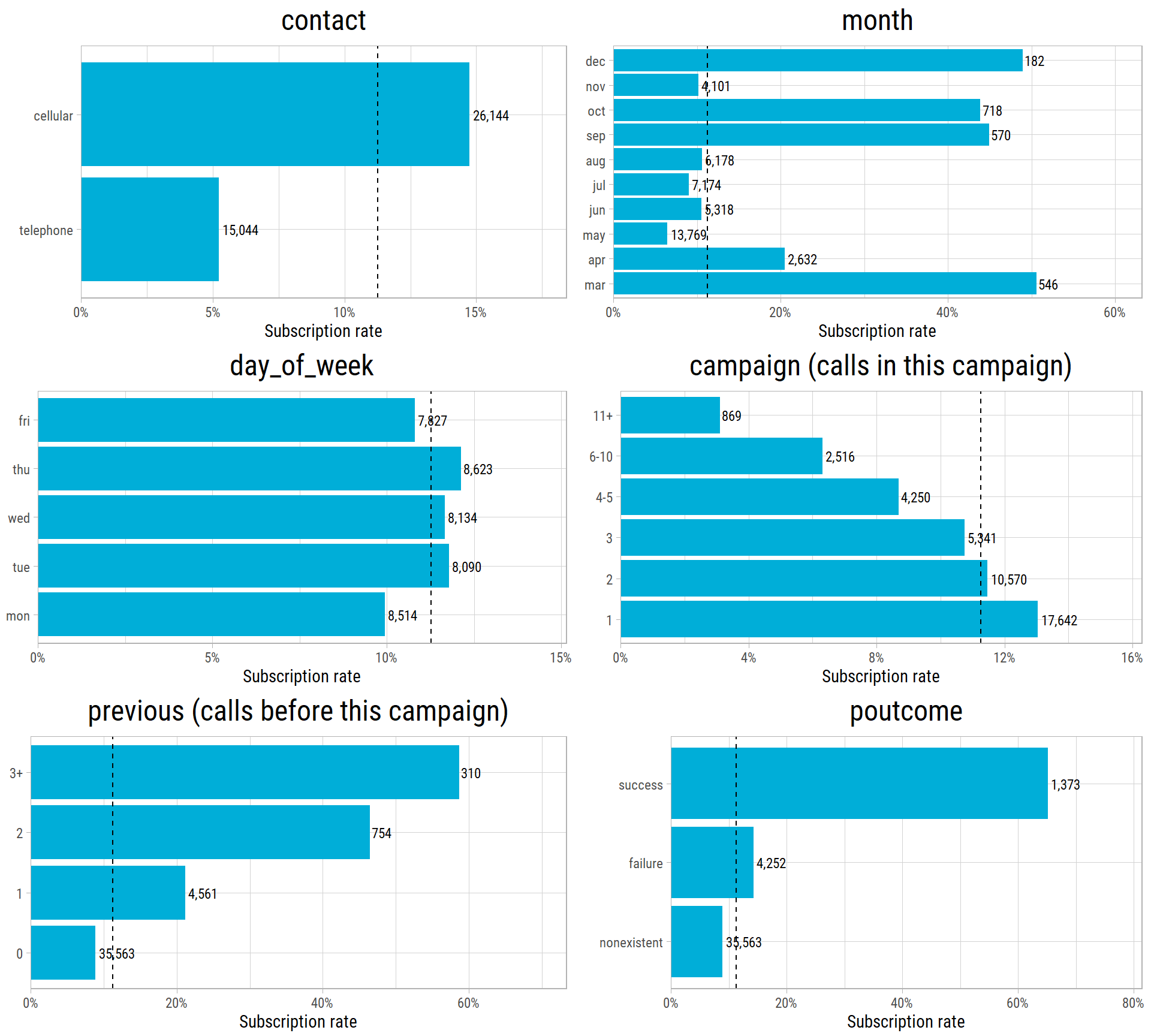
What’s notable?
- Clients called on a cell phone subscribe almost three times as often as clients called on a landline.
- The months with the fewest calls (March, September, October and December) have the highest rates, close to 50%. May, the busiest month, has the lowest rate. We look at this again in the next section.
- The day of the week makes little difference.
- Each extra call in the same campaign makes a yes less likely. Only 3% of the clients who were called more than 10 times subscribed.
- The more often a client was called in previous campaigns, the more likely a yes: these clients already know the bank.
- The result of the previous campaign is the strongest client-level signal: 65% of the clients who said yes before said yes again.
The Economy and the Time of the Call
The rows are in the order of the calls. So we can follow the subscription rate over time. Here, we split the calls into blocks of 1,000 consecutive calls:
dfTime <- dfRaw %>%
  mutate(call_order = row_number(), block = (call_order - 1) %/% 1000 + 1) %>%
  group_by(block) %>%
  summarise(first_call = min(call_order), rate = mean(y == "yes"), euribor3m = mean(euribor3m), nr.employed = mean(nr.employed))

p1 <- ggplot(dfTime, aes(x = first_call, y = rate)) +
  geom_line(color = "#00AED8") + geom_point(color = "#00AED8") +
  scale_y_continuous(labels = scales::label_percent()) +
  scale_x_continuous(labels = scales::label_comma()) +
  labs(x = NULL, y = "Subscription rate", title = "Subscription rate in each block of 1,000 calls")
p2 <- ggplot(dfTime, aes(x = first_call, y = euribor3m)) +
  geom_line(color = "#F37735") + geom_point(color = "#F37735") +
  scale_x_continuous(labels = scales::label_comma()) +
  labs(x = "Call number (in order of time)", y = "3 month Euribor (%)", title = "Interest rate at the time of the calls")
cowplot::plot_grid(plotlist = list(p1, p2), ncol = 1, align = "v")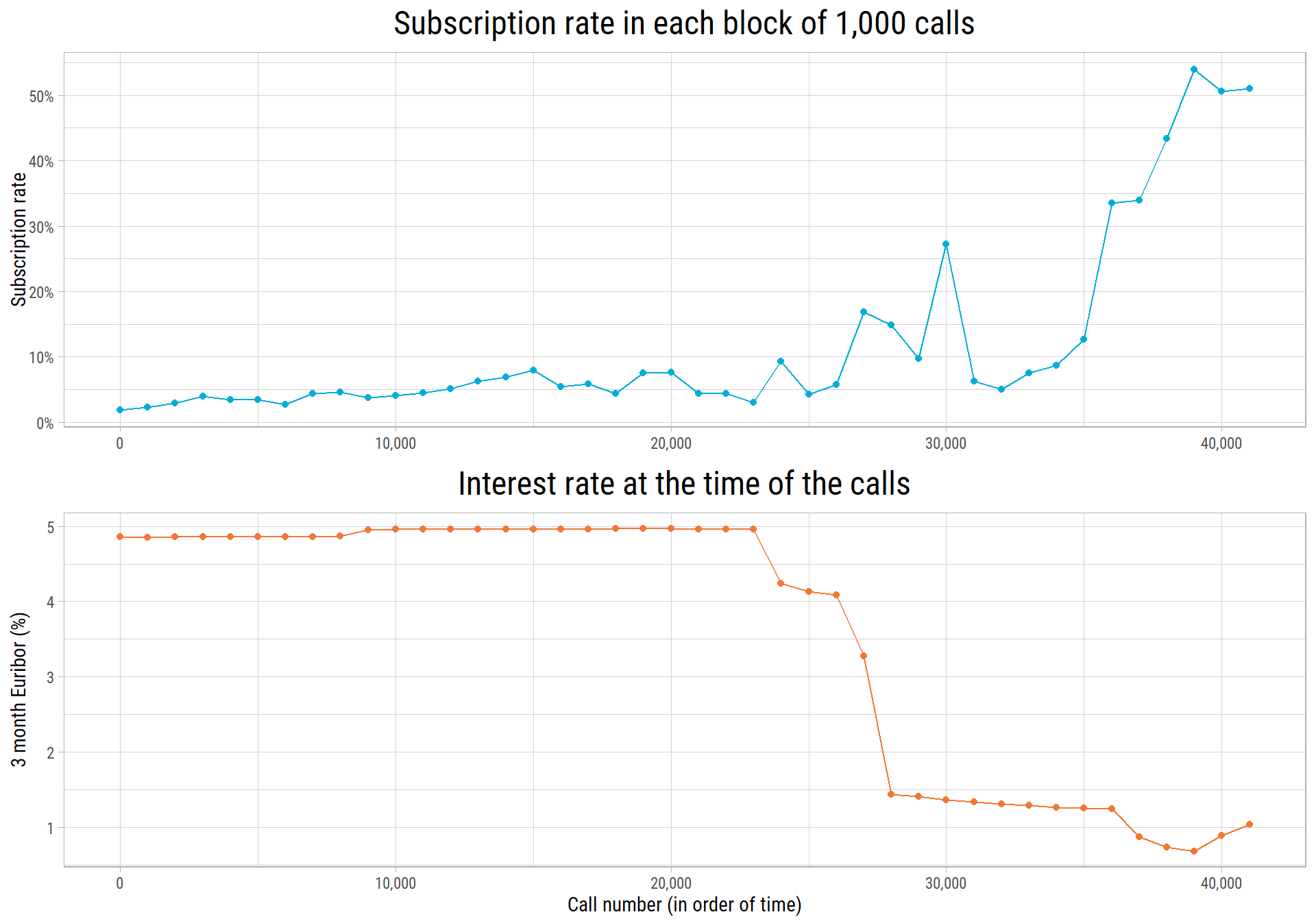
eda_plot_correlation_matrix(dfRaw %>% select(emp.var.rate, cons.price.idx, cons.conf.idx, euribor3m, nr.employed),
                            plotTitle = "Correlation of the economic features")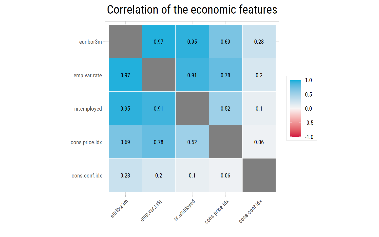
What’s notable?
- In the first 23,000 or so calls, fewer than 1 in 10 calls ended with a yes. After the interest rate fell in late 2008 and 2009, the rate rose, and in the last blocks about half of the calls were successful. Fewer calls were made in that period, which explains why the quiet months had the highest rates.
euribor3m,emp.var.rateandnr.employedmove together (their correlations are above 0.9). They describe the same economic cycle.- So the economic features are strong predictors, but much of their power comes from telling the model when the call was made. A model can learn that calls in a certain period were successful. That is useful when we predict calls from the same period, but the economy of the next campaign will be different. In Part 2, we test the models on calls from the same period, and then on later calls.
Associations Between Features
Correlation only works for numerical features. To compare all the features at once, including the categorical ones and the target, we use an association matrix. It uses Cramér’s V for pairs of categorical features: 0 means no association and 1 means that one feature completely determines the other.
dfAssoc <- dfRaw %>%
  select(-duration) %>%
  mutate(across(where(is.character), as.factor))
eda_plot_association_matrix(dfAssoc, outlineVar = "y", plotTitle = "Association of features with each other and with y")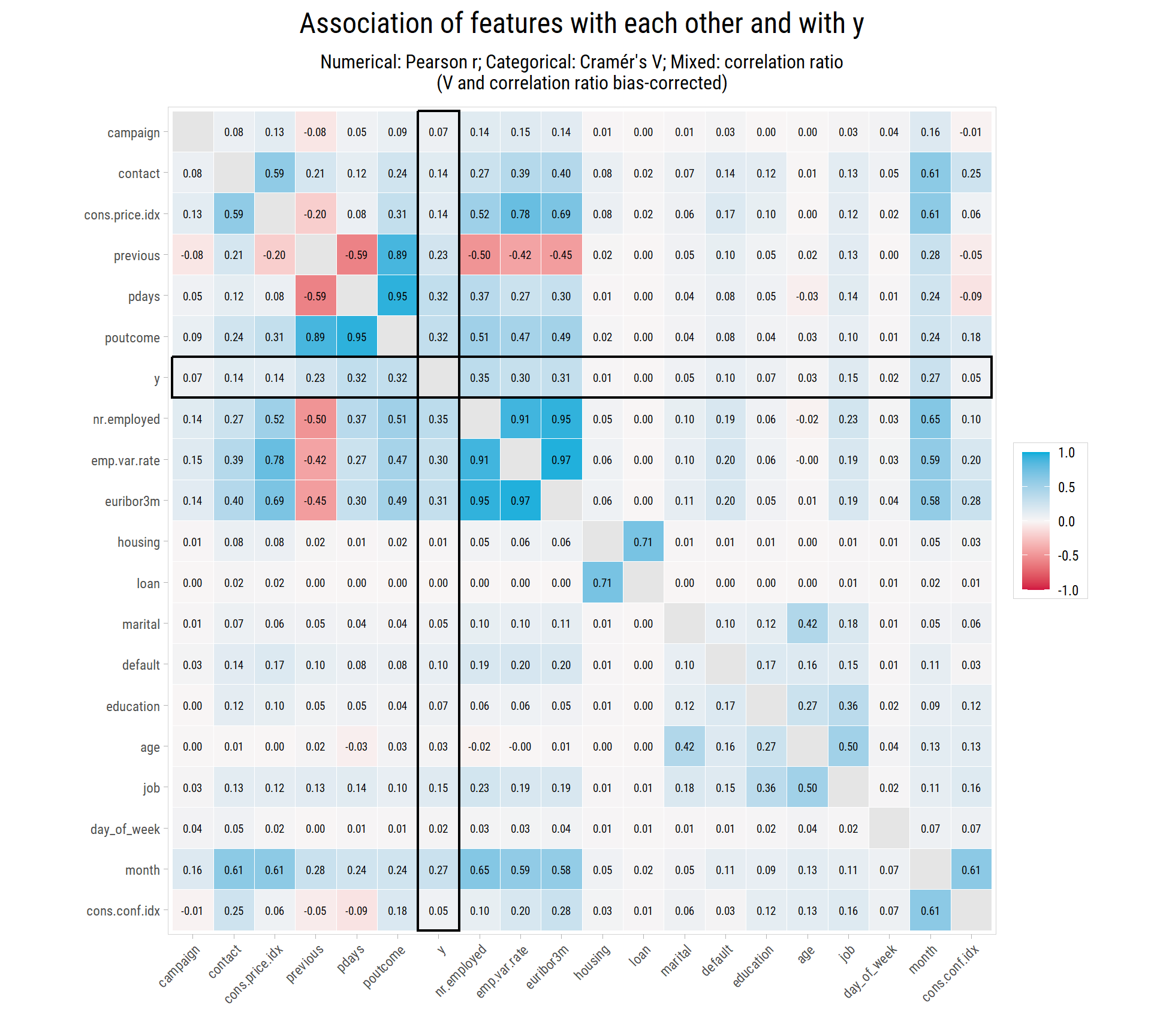
What’s notable?
- The target
yis most strongly associated with the economic features (about 0.3), withpoutcome,pdaysandprevious(the history of previous campaigns), and withmonth.jobandcontactfollow, with about 0.15. pdays,previousandpoutcomeare strongly associated with each other, because they all describe the previous campaign.month,contactand the economic features are strongly associated with each other, because they all depend on when the call was made.ageis associated withjobandmarital: students are young, and retired people are old.housingandloanare almost unrelated toy. They are associated with each other only because their unknown values are the same clients.
Preparing the Data for Models
Based on what we have found, we make these changes:
- Remove the 12 duplicate rows.
- Drop
duration, which is not known before a call (data leakage). - Replace
pdayswith a yes/no feature,recent_contact, that says whetherpdayswas recorded. Its exact value adds little, because it is recorded almost only for clients with a successful previous campaign, and the value 999 would mislead a linear model. - Change the 3 yes answers in
defaultto unknown, so that the feature compares clients who said no with all the others. Three examples are too few for a model to learn from. - Keep unknown as a category in the other features, because it is informative: for example, clients whose education is unknown subscribe more often than average.
- Put the months and the days of the week in calendar order.
- Add an
Idthat keeps the order of the calls, so that in Part 2 we can test the models on later calls. The models do not use it as a feature.
Then we set aside 25% of the calls as a testing set, which the models will not see while they learn. We use stratified sampling, so that the testing set has the same subscription rate as the training set.
dfClean <- dfRaw %>%
  mutate(Id = row_number()) %>%
  filter(!duplicated(pick(-Id))) %>%
  select(-duration) %>%
  mutate(recent_contact = if_else(pdays != 999, "yes", "no"),
         default = if_else(default == "yes", "unknown", default),
         month = factor(month, levels = c("mar","apr","may","jun","jul","aug","sep","oct","nov","dec")),
         day_of_week = factor(day_of_week, levels = c("mon","tue","wed","thu","fri")),
         y = factor(y, levels = c("yes", "no"))) %>%
  select(-pdays) %>%
  mutate(across(where(is.character), as.factor)) %>%
  select(Id, y, everything())

vFeaturesNum <- dfClean %>% select(-Id, -y) %>% select(where(is.numeric)) %>% colnames()
vFeaturesCat <- dfClean %>% select(-Id, -y) %>% select(where(is.factor)) %>% colnames()

# stratified split into training (75%) and testing (25%) sets
set.seed(2300)
data_split <- initial_split(dfClean, prop = 0.75, strata = y)
vTestIDs <- testing(data_split)$Id

dfSplit <- dfClean %>%
  mutate(set = if_else(Id %in% vTestIDs, "testing", "training")) %>%
  group_by(set) %>%
  summarise(calls = n(), subscribed = sum(y == "yes"), rate = round(100 * mean(y == "yes"), 2))
knitr::kable(dfSplit, col.names = c("Set", "Calls", "Subscribed", "Subscription rate (%)"))| Set | Calls | Subscribed | Subscription rate (%) |
|---|---|---|---|
| testing | 10295 | 1160 | 11.27 |
| training | 30881 | 3479 | 11.27 |
save(dfClean, vTestIDs, vFeaturesNum, vFeaturesCat, file = "Bank_Marketing_Clean.Rda")The finalized dataset has 41,176 calls and 19 features: 8 numerical and 11 categorical.
Next Steps
We have learned that:
- The history of a client with the bank (
poutcome,previous) and the type of phone are strong signals. - The economy and the time of the call matter a lot, so we must be careful about how we test the models.
- Age and job matter, but less.
durationmust not be used, even though it looks like the best predictor.
In Part 2, we use this dataset to build models that predict which clients will subscribe.