Ames Housing - Part 1 - Laying the foundation - Building a Data Pipeline
Other posts in this series:
- Ames Housing - Part 2 - Walkthrough - An Exploratory Data Analysis
- Ames Housing - Part 3 - Closing the deal - Building Models
In this case study, we use the Ames Housing dataset to predict the sale prices of houses. The case study has three posts:
- In this post, we build a data pipeline: a series of steps that fixes errors in the data, fills in missing values, creates new features and drops features that we do not need. At the end, we save the finalized dataset.
- In Part 2, we explore the finalized dataset to find which features affect the sale price.
- In Part 3, we build models that predict the prices. A model is a formula that a computer learns from examples.
Neighborhoods of Ames
Location is very important for the price of a house. The version of the dataset that we use (from Kaggle) does not have the location of each property. But the full dataset by Dean De Cock, which is in the R package modeldata, has the latitude and longitude of 2930 properties. We use it to show where the neighborhoods are.
On this map, each dot is a property. The color shows the type of its neighborhood. Later in this post, we put the neighborhoods into five types by their median sale price: Type1 has the most expensive neighborhoods, and Type5 has the cheapest. The labels show the short names of the neighborhoods that the dataset uses. You can zoom in, move the map, and click a label to see the details of a neighborhood:
library(leaflet)

# Neighborhood types, from the most expensive (Type1) to the cheapest (Type5), by median SalePrice.
# The same groups are used to create NeighborhoodType later in this post.
lNeighborhoodTypes <- list(Type1 = c("StoneBr", "NridgHt", "NoRidge"),
                           Type2 = c("Veenker", "Timber", "Somerst"),
                           Type3 = c("Crawfor", "CollgCr", "ClearCr", "Blmngtn", "Gilbert", "NWAmes", "SawyerW"),
                           Type4 = c("Mitchel", "NPkVill", "NAmes", "SWISU", "Sawyer", "Blueste", "BrkSide", "Edwards", "OldTown"),
                           Type5 = c("IDOTRR", "BrDale", "MeadowV"))

# modeldata::ames spells out the neighborhood names; this dataset uses short codes
dfNeighborhoodNames <- tribble(
  ~Name,                                     ~Code,
  "Bloomington_Heights",                     "Blmngtn",
  "Blueste",                                 "Blueste",
  "Briardale",                               "BrDale",
  "Brookside",                               "BrkSide",
  "Clear_Creek",                             "ClearCr",
  "College_Creek",                           "CollgCr",
  "Crawford",                                "Crawfor",
  "Edwards",                                 "Edwards",
  "Gilbert",                                 "Gilbert",
  "Iowa_DOT_and_Rail_Road",                  "IDOTRR",
  "Meadow_Village",                          "MeadowV",
  "Mitchell",                                "Mitchel",
  "North_Ames",                              "NAmes",
  "Northridge",                              "NoRidge",
  "Northpark_Villa",                         "NPkVill",
  "Northridge_Heights",                      "NridgHt",
  "Northwest_Ames",                          "NWAmes",
  "Old_Town",                                "OldTown",
  "South_and_West_of_Iowa_State_University", "SWISU",
  "Sawyer",                                  "Sawyer",
  "Sawyer_West",                             "SawyerW",
  "Somerset",                                "Somerst",
  "Stone_Brook",                             "StoneBr",
  "Timberland",                              "Timber",
  "Veenker",                                 "Veenker") %>%
  mutate(Type = map_chr(Code, function(code) names(lNeighborhoodTypes)[map_lgl(lNeighborhoodTypes, ~ code %in% .x)]))

# properties with their location; neighborhoods that are not in this dataset are left out
dfLocations <- modeldata::ames %>%
  transmute(Name = as.character(Neighborhood), Longitude, Latitude, SalePrice = Sale_Price) %>%
  inner_join(dfNeighborhoodNames, by = "Name") %>%
  mutate(Type = factor(Type, levels = names(lNeighborhoodTypes)))
nLeftOut <- nrow(modeldata::ames) - nrow(dfLocations)

# one label per neighborhood, at the median location of its properties
dfCenters <- dfLocations %>%
  group_by(Name, Code, Type) %>%
  summarise(Longitude = median(Longitude), Latitude = median(Latitude),
            Properties = n(), MedianPrice = median(SalePrice), .groups = "drop") %>%
  mutate(Popup = glue::glue("<b>{Code}</b>: {str_replace_all(Name, '_', ' ')}<br>",
                            "Neighborhood type: {Type}<br>",
                            "Properties: {Properties}<br>",
                            "Median sale price: {scales::dollar(MedianPrice)}"))

palType <- colorFactor(quant_pal("metro")(5), domain = levels(dfLocations$Type))

leaflet(dfLocations, width = "100%", height = 600) %>%
  addTiles() %>%
  addCircleMarkers(~Longitude, ~Latitude, color = ~palType(Type), radius = 3, stroke = FALSE, fillOpacity = 0.6) %>%
  addCircleMarkers(data = dfCenters, ~Longitude, ~Latitude, popup = ~Popup, radius = 6,
                   color = "white", weight = 1, fillColor = ~palType(Type), fillOpacity = 1,
                   label = ~Code, labelOptions = labelOptions(noHide = TRUE, direction = "right", textOnly = TRUE,
                                                              style = list("font-weight" = "bold", "font-size" = "12px", "color" = "#222",
                                                                           "text-shadow" = "0 0 3px #fff, 0 0 3px #fff"))) %>%
addLegend("bottomright", pal = palType, values = ~Type, title = "Neighborhood type", opacity = 1)- All three of the most expensive neighborhoods (Type1) are in the north of the city.
- The other types are spread across the city. For example, the cheapest type (Type5) has BrDale in the north, IDOTRR near the center and MeadowV in the south. And Timber, a Type2 neighborhood, is in the far south of the city, like Mitchel (Type4) and MeadowV (Type5). So the part of the city alone does not decide the price: neighborhoods that are close to each other can have very different prices.
- 11 properties of the full dataset are in neighborhoods that our dataset does not have, so the map does not show them.
Data Summaries
The Ames Housing dataset has the sale prices of properties in Ames, Iowa, and 80 other attributes of each property. We call each attribute a feature. Each property has an Id number. The data comes in two parts: a training set and a testing set. Here are the number of rows (properties) and columns (features) in each set:
print("Dimensions of the training set")[1] "Dimensions of the training set"dim(dfTrain)[1] 1460 81vTrainIDs <- dfTrain$Id
print("Dimensions of the testing set")[1] "Dimensions of the testing set"dim(dfTest)[1] 1459 81vTestIDs <- dfTest$Id
dfClean <- dfTrain %>% bind_rows(dfTest)The data description explains each feature, and the meaning of each category. It is long, so it is folded:
# data_description.txt has one line "Feature: description" for each feature,
# followed by one line "code<TAB>meaning" for each of its categories, if it has any
vLines <- readLines("data_description.txt")
vStarts <- grep("^[[:alnum:]]+:", vLines)
vEnds <- c(vStarts[-1] - 1, length(vLines))

dfDescription <- map2_dfr(vStarts, vEnds, function(iStart, iEnd) {
  vParts <- str_split_fixed(vLines[iStart], ":", 2)
  vCategories <- trimws(vLines[seq_len(iEnd - iStart) + iStart])
  vCategories <- vCategories[vCategories != ""]
  vCodes <- str_split_fixed(vCategories, "	", 2)
  tibble(Feature = vParts[1],
         Description = trimws(vParts[2]),
         Categories = if (length(vCategories) > 0) paste0("<b>", trimws(vCodes[, 1]), "</b>: ", trimws(vCodes[, 2]), collapse = "<br>") else "")
})

cat('<details class="code-fold"><summary>Show the data description</summary>

')
Show the data description
cat(knitr::kable(dfDescription, format = "html", escape = FALSE), sep = "
")| Feature | Description | Categories |
|---|---|---|
| MSSubClass | Identifies the type of dwelling involved in the sale. |
20: 1-STORY 1946 & NEWER ALL STYLES 30: 1-STORY 1945 & OLDER 40: 1-STORY W/FINISHED ATTIC ALL AGES 45: 1-1/2 STORY - UNFINISHED ALL AGES 50: 1-1/2 STORY FINISHED ALL AGES 60: 2-STORY 1946 & NEWER 70: 2-STORY 1945 & OLDER 75: 2-1/2 STORY ALL AGES 80: SPLIT OR MULTI-LEVEL 85: SPLIT FOYER 90: DUPLEX - ALL STYLES AND AGES 120: 1-STORY PUD (Planned Unit Development) - 1946 & NEWER 150: 1-1/2 STORY PUD - ALL AGES 160: 2-STORY PUD - 1946 & NEWER 180: PUD - MULTILEVEL - INCL SPLIT LEV/FOYER 190: 2 FAMILY CONVERSION - ALL STYLES AND AGES |
| MSZoning | Identifies the general zoning classification of the sale. |
A: Agriculture C: Commercial FV: Floating Village Residential I: Industrial RH: Residential High Density RL: Residential Low Density RP: Residential Low Density Park RM: Residential Medium Density |
| LotFrontage | Linear feet of street connected to property | |
| LotArea | Lot size in square feet | |
| Street | Type of road access to property |
Grvl: Gravel Pave: Paved |
| Alley | Type of alley access to property |
Grvl: Gravel Pave: Paved NA: No alley access |
| LotShape | General shape of property |
Reg: Regular IR1: Slightly irregular IR2: Moderately Irregular IR3: Irregular |
| LandContour | Flatness of the property |
Lvl: Near Flat/Level Bnk: Banked - Quick and significant rise from street grade to building HLS: Hillside - Significant slope from side to side Low: Depression |
| Utilities | Type of utilities available |
AllPub: All public Utilities (E,G,W,& S) NoSewr: Electricity, Gas, and Water (Septic Tank) NoSeWa: Electricity and Gas Only ELO: Electricity only |
| LotConfig | Lot configuration |
Inside: Inside lot Corner: Corner lot CulDSac: Cul-de-sac FR2: Frontage on 2 sides of property FR3: Frontage on 3 sides of property |
| LandSlope | Slope of property |
Gtl: Gentle slope Mod: Moderate Slope Sev: Severe Slope |
| Neighborhood | Physical locations within Ames city limits |
Blmngtn: Bloomington Heights Blueste: Bluestem BrDale: Briardale BrkSide: Brookside ClearCr: Clear Creek CollgCr: College Creek Crawfor: Crawford Edwards: Edwards Gilbert: Gilbert IDOTRR: Iowa DOT and Rail Road MeadowV: Meadow Village Mitchel: Mitchell Names: North Ames NoRidge: Northridge NPkVill: Northpark Villa NridgHt: Northridge Heights NWAmes: Northwest Ames OldTown: Old Town SWISU: South & West of Iowa State University Sawyer: Sawyer SawyerW: Sawyer West Somerst: Somerset StoneBr: Stone Brook Timber: Timberland Veenker: Veenker |
| Condition1 | Proximity to various conditions |
Artery: Adjacent to arterial street Feedr: Adjacent to feeder street Norm: Normal RRNn: Within 200’ of North-South Railroad RRAn: Adjacent to North-South Railroad PosN: Near positive off-site feature–park, greenbelt, etc. PosA: Adjacent to postive off-site feature RRNe: Within 200’ of East-West Railroad RRAe: Adjacent to East-West Railroad |
| Condition2 | Proximity to various conditions (if more than one is present) |
Artery: Adjacent to arterial street Feedr: Adjacent to feeder street Norm: Normal RRNn: Within 200’ of North-South Railroad RRAn: Adjacent to North-South Railroad PosN: Near positive off-site feature–park, greenbelt, etc. PosA: Adjacent to postive off-site feature RRNe: Within 200’ of East-West Railroad RRAe: Adjacent to East-West Railroad |
| BldgType | Type of dwelling |
1Fam: Single-family Detached 2FmCon: Two-family Conversion; originally built as one-family dwelling Duplx: Duplex TwnhsE: Townhouse End Unit TwnhsI: Townhouse Inside Unit |
| HouseStyle | Style of dwelling |
1Story: One story 1.5Fin: One and one-half story - 2nd level finished 1.5Unf: One and one-half story - 2nd level unfinished 2Story: Two story 2.5Fin: Two and one-half story - 2nd level finished 2.5Unf: Two and one-half story - 2nd level unfinished SFoyer: Split Foyer SLvl: Split Level |
| OverallQual | Rates the overall material and finish of the house |
10: Very Excellent 9: Excellent 8: Very Good 7: Good 6: Above Average 5: Average 4: Below Average 3: Fair 2: Poor 1: Very Poor |
| OverallCond | Rates the overall condition of the house |
10: Very Excellent 9: Excellent 8: Very Good 7: Good 6: Above Average 5: Average 4: Below Average 3: Fair 2: Poor 1: Very Poor |
| YearBuilt | Original construction date | |
| YearRemodAdd | Remodel date (same as construction date if no remodeling or additions) | |
| RoofStyle | Type of roof |
Flat: Flat Gable: Gable Gambrel: Gabrel (Barn) Hip: Hip Mansard: Mansard Shed: Shed |
| RoofMatl | Roof material |
ClyTile: Clay or Tile CompShg: Standard (Composite) Shingle Membran: Membrane Metal: Metal Roll: Roll Tar&Grv: Gravel & Tar WdShake: Wood Shakes WdShngl: Wood Shingles |
| Exterior1st | Exterior covering on house |
AsbShng: Asbestos Shingles AsphShn: Asphalt Shingles BrkComm: Brick Common BrkFace: Brick Face CBlock: Cinder Block CemntBd: Cement Board HdBoard: Hard Board ImStucc: Imitation Stucco MetalSd: Metal Siding Other: Other Plywood: Plywood PreCast: PreCast Stone: Stone Stucco: Stucco VinylSd: Vinyl Siding Wd Sdng: Wood Siding WdShing: Wood Shingles |
| Exterior2nd | Exterior covering on house (if more than one material) |
AsbShng: Asbestos Shingles AsphShn: Asphalt Shingles BrkComm: Brick Common BrkFace: Brick Face CBlock: Cinder Block CemntBd: Cement Board HdBoard: Hard Board ImStucc: Imitation Stucco MetalSd: Metal Siding Other: Other Plywood: Plywood PreCast: PreCast Stone: Stone Stucco: Stucco VinylSd: Vinyl Siding Wd Sdng: Wood Siding WdShing: Wood Shingles |
| MasVnrType | Masonry veneer type |
BrkCmn: Brick Common BrkFace: Brick Face CBlock: Cinder Block None: None Stone: Stone |
| MasVnrArea | Masonry veneer area in square feet | |
| ExterQual | Evaluates the quality of the material on the exterior |
Ex: Excellent Gd: Good TA: Average/Typical Fa: Fair Po: Poor |
| ExterCond | Evaluates the present condition of the material on the exterior |
Ex: Excellent Gd: Good TA: Average/Typical Fa: Fair Po: Poor |
| Foundation | Type of foundation |
BrkTil: Brick & Tile CBlock: Cinder Block PConc: Poured Contrete Slab: Slab Stone: Stone Wood: Wood |
| BsmtQual | Evaluates the height of the basement |
Ex: Excellent (100+ inches) Gd: Good (90-99 inches) TA: Typical (80-89 inches) Fa: Fair (70-79 inches) Po: Poor (<70 inches NA: No Basement |
| BsmtCond | Evaluates the general condition of the basement |
Ex: Excellent Gd: Good TA: Typical - slight dampness allowed Fa: Fair - dampness or some cracking or settling Po: Poor - Severe cracking, settling, or wetness NA: No Basement |
| BsmtExposure | Refers to walkout or garden level walls |
Gd: Good Exposure Av: Average Exposure (split levels or foyers typically score average or above) Mn: Mimimum Exposure No: No Exposure NA: No Basement |
| BsmtFinType1 | Rating of basement finished area |
GLQ: Good Living Quarters ALQ: Average Living Quarters BLQ: Below Average Living Quarters Rec: Average Rec Room LwQ: Low Quality Unf: Unfinshed NA: No Basement |
| BsmtFinSF1 | Type 1 finished square feet | |
| BsmtFinType2 | Rating of basement finished area (if multiple types) |
GLQ: Good Living Quarters ALQ: Average Living Quarters BLQ: Below Average Living Quarters Rec: Average Rec Room LwQ: Low Quality Unf: Unfinshed NA: No Basement |
| BsmtFinSF2 | Type 2 finished square feet | |
| BsmtUnfSF | Unfinished square feet of basement area | |
| TotalBsmtSF | Total square feet of basement area | |
| Heating | Type of heating |
Floor: Floor Furnace GasA: Gas forced warm air furnace GasW: Gas hot water or steam heat Grav: Gravity furnace OthW: Hot water or steam heat other than gas Wall: Wall furnace |
| HeatingQC | Heating quality and condition |
Ex: Excellent Gd: Good TA: Average/Typical Fa: Fair Po: Poor |
| CentralAir | Central air conditioning |
N: No Y: Yes |
| Electrical | Electrical system |
SBrkr: Standard Circuit Breakers & Romex FuseA: Fuse Box over 60 AMP and all Romex wiring (Average) FuseF: 60 AMP Fuse Box and mostly Romex wiring (Fair) FuseP: 60 AMP Fuse Box and mostly knob & tube wiring (poor) Mix: Mixed |
| 1stFlrSF | First Floor square feet | |
| 2ndFlrSF | Second floor square feet | |
| LowQualFinSF | Low quality finished square feet (all floors) | |
| GrLivArea | Above grade (ground) living area square feet | |
| BsmtFullBath | Basement full bathrooms | |
| BsmtHalfBath | Basement half bathrooms | |
| FullBath | Full bathrooms above grade | |
| HalfBath | Half baths above grade | |
| Bedroom | Bedrooms above grade (does NOT include basement bedrooms) | |
| KitchenAbvGr | Kitchens above grade | |
| KitchenQual | Kitchen quality |
Ex: Excellent Gd: Good TA: Typical/Average Fa: Fair Po: Poor |
| TotRmsAbvGrd | Total rooms above grade (does not include bathrooms) | |
| Functional | Home functionality (Assume typical unless deductions are warranted) |
Typ: Typical Functionality Min1: Minor Deductions 1 Min2: Minor Deductions 2 Mod: Moderate Deductions Maj1: Major Deductions 1 Maj2: Major Deductions 2 Sev: Severely Damaged Sal: Salvage only |
| Fireplaces | Number of fireplaces | |
| FireplaceQu | Fireplace quality |
Ex: Excellent - Exceptional Masonry Fireplace Gd: Good - Masonry Fireplace in main level TA: Average - Prefabricated Fireplace in main living area or Masonry Fireplace in basement Fa: Fair - Prefabricated Fireplace in basement Po: Poor - Ben Franklin Stove NA: No Fireplace |
| GarageType | Garage location |
2Types: More than one type of garage Attchd: Attached to home Basment: Basement Garage BuiltIn: Built-In (Garage part of house - typically has room above garage) CarPort: Car Port Detchd: Detached from home NA: No Garage |
| GarageYrBlt | Year garage was built | |
| GarageFinish | Interior finish of the garage |
Fin: Finished RFn: Rough Finished Unf: Unfinished NA: No Garage |
| GarageCars | Size of garage in car capacity | |
| GarageArea | Size of garage in square feet | |
| GarageQual | Garage quality |
Ex: Excellent Gd: Good TA: Typical/Average Fa: Fair Po: Poor NA: No Garage |
| GarageCond | Garage condition |
Ex: Excellent Gd: Good TA: Typical/Average Fa: Fair Po: Poor NA: No Garage |
| PavedDrive | Paved driveway |
Y: Paved P: Partial Pavement N: Dirt/Gravel |
| WoodDeckSF | Wood deck area in square feet | |
| OpenPorchSF | Open porch area in square feet | |
| EnclosedPorch | Enclosed porch area in square feet | |
| 3SsnPorch | Three season porch area in square feet | |
| ScreenPorch | Screen porch area in square feet | |
| PoolArea | Pool area in square feet | |
| PoolQC | Pool quality |
Ex: Excellent Gd: Good TA: Average/Typical Fa: Fair NA: No Pool |
| Fence | Fence quality |
GdPrv: Good Privacy MnPrv: Minimum Privacy GdWo: Good Wood MnWw: Minimum Wood/Wire NA: No Fence |
| MiscFeature | Miscellaneous feature not covered in other categories |
Elev: Elevator Gar2: 2nd Garage (if not described in garage section) Othr: Other Shed: Shed (over 100 SF) TenC: Tennis Court NA: None |
| MiscVal | $Value of miscellaneous feature | |
| MoSold | Month Sold (MM) | |
| YrSold | Year Sold (YYYY) | |
| SaleType | Type of sale |
WD: Warranty Deed - Conventional CWD: Warranty Deed - Cash VWD: Warranty Deed - VA Loan New: Home just constructed and sold COD: Court Officer Deed/Estate Con: Contract 15% Down payment regular terms ConLw: Contract Low Down payment and low interest ConLI: Contract Low Interest ConLD: Contract Low Down Oth: Other |
| SaleCondition | Condition of sale |
Normal: Normal Sale Abnorml: Abnormal Sale - trade, foreclosure, short sale AdjLand: Adjoining Land Purchase Alloca: Allocation - two linked properties with separate deeds, typically condo with a garage unit Family: Sale between family members Partial: Home was not completed when last assessed (associated with New Homes) |
cat("
</details>
")
Now, let’s put the training set and the testing set together in one dataset, and count the missing values in each feature:
eda_plot_missing_counts(dfClean)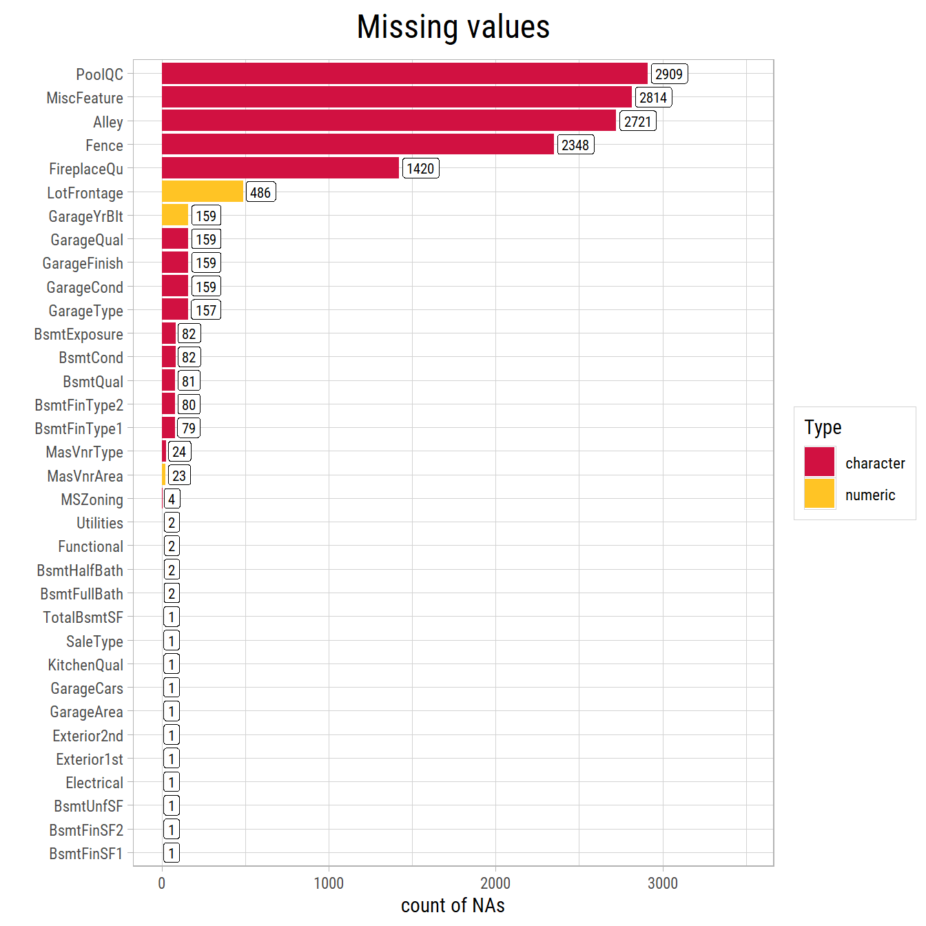
What’s notable?
- The combined dataset has 2919 properties.
- Very few properties have a pool, a fence or access to an alley.
- Very few properties have a special feature that other features do not describe (
MiscFeature). - More than 12 features have at least 1 missing value. The dataset is small, so we do not want to remove properties. Instead, we fill in each missing value with a likely value. This is called imputation.
Data Cleaning & Transformation
In this section, we look at the features of the complete dataset, and we make a set of steps to clean the data.
Fixing Data Errors
First, we check that the data makes sense:
YearRemodAdd(the year of the last remodel) must not be earlier thanYearBuilt: 1 property to fixYrSold(the year of the sale) must not be earlier thanYearRemodAdd: 3 properties to fix
dfClean %>% select(Id, YearBuilt, YearRemodAdd, YrSold) %>% dplyr::filter(YearRemodAdd < YearBuilt)# A tibble: 1 × 4
Id YearBuilt YearRemodAdd YrSold
<dbl> <dbl> <dbl> <dbl>
1 1877 2002 2001 2009dfClean %>% select(Id, YearBuilt, YearRemodAdd, YrSold) %>% dplyr::filter(YrSold < YearRemodAdd)# A tibble: 3 × 4
Id YearBuilt YearRemodAdd YrSold
<dbl> <dbl> <dbl> <dbl>
1 524 2007 2008 2007
2 2296 2007 2008 2007
3 2550 2008 2009 2007# fix errors
dfClean <- dfClean %>%
mutate(YearRemodAdd = ifelse(YearRemodAdd < YearBuilt, YearBuilt, YearRemodAdd)) %>%
mutate(YrSold = ifelse(YrSold < YearRemodAdd, YearRemodAdd, YrSold))GarageYrBlt(the year the garage was built) must not be earlier thanYearBuilt: 18 properties to fixGarageYrBltmust not be later thanYrSold: 1 property to fix
dfClean %>% select(Id, YearBuilt, GarageYrBlt, YrSold) %>% dplyr::filter(GarageYrBlt < YearBuilt)# A tibble: 18 × 4
Id YearBuilt GarageYrBlt YrSold
<dbl> <dbl> <dbl> <dbl>
1 30 1927 1920 2008
2 94 1910 1900 2007
3 325 1967 1961 2010
4 601 2005 2003 2006
5 737 1950 1949 2006
6 1104 1959 1954 2006
7 1377 1930 1925 2008
8 1415 1923 1922 2008
9 1419 1963 1962 2008
10 1522 1959 1956 2010
11 1577 2010 2009 2010
12 1806 1935 1920 2009
13 1841 1978 1960 2009
14 1896 1941 1940 2009
15 1898 1935 1926 2009
16 2123 1945 1925 2008
17 2264 2006 2005 2007
18 2510 2006 2005 2007dfClean %>% select(Id, YearBuilt, GarageYrBlt, YrSold) %>% dplyr::filter(GarageYrBlt > YrSold)# A tibble: 1 × 4
Id YearBuilt GarageYrBlt YrSold
<dbl> <dbl> <dbl> <dbl>
1 2593 2006 2207 2007# fix errors
dfClean <- dfClean %>%
mutate(GarageYrBlt = ifelse(GarageYrBlt < YearBuilt, YearBuilt, GarageYrBlt)) %>%
mutate(GarageYrBlt = ifelse(GarageYrBlt > YrSold, YrSold, GarageYrBlt))Imputing Missing Values & New Features
Basement Features
For one property (
Id= 2121), all the basement features are missing (NA). We setTotalBsmtSF(the total basement area) to 0.Now 79 properties have no basement (
TotalBsmtSF= 0). For these properties, we change all the missing basement values to None.The quality of basements is different in different neighborhoods. So we fill in each remaining missing value with the most common value in the same
Neighborhood.
# 1. Change TotalBsmtSF to 0 when all basement features are NA
#####################################################################################################################
dfClean %>% select(Id, Neighborhood, contains("Bsmt")) %>% dplyr::filter(is.na(TotalBsmtSF))
# A tibble: 1 × 13
Id Neighborhood BsmtQual BsmtCond BsmtExposure BsmtFinType1 BsmtFinSF1 BsmtFinType2 BsmtFinSF2 BsmtUnfSF TotalBsmtSF BsmtFullBath BsmtHalfBath
<dbl> <chr> <chr> <chr> <chr> <chr> <dbl> <chr> <dbl> <dbl> <dbl> <dbl> <dbl>
1 2121 BrkSide <NA> <NA> <NA> <NA> NA <NA> NA NA NA NA NAdfClean <- dfClean %>% mutate(TotalBsmtSF = if_else(Id == 2121, 0, TotalBsmtSF))
# 2. Change NA values to None or 0 if there is no basement
#####################################################################################################################
dfClean %>% select(Id, Neighborhood, contains("Bsmt")) %>% dplyr::filter(TotalBsmtSF == 0)# A tibble: 79 × 13
Id Neighborhood BsmtQual BsmtCond BsmtExposure BsmtFinType1 BsmtFinSF1 BsmtFinType2 BsmtFinSF2 BsmtUnfSF TotalBsmtSF BsmtFullBath BsmtHalfBath
<dbl> <chr> <chr> <chr> <chr> <chr> <dbl> <chr> <dbl> <dbl> <dbl> <dbl> <dbl>
1 18 Sawyer <NA> <NA> <NA> <NA> 0 <NA> 0 0 0 0 0
2 40 Edwards <NA> <NA> <NA> <NA> 0 <NA> 0 0 0 0 0
3 91 NAmes <NA> <NA> <NA> <NA> 0 <NA> 0 0 0 0 0
4 103 SawyerW <NA> <NA> <NA> <NA> 0 <NA> 0 0 0 0 0
5 157 NAmes <NA> <NA> <NA> <NA> 0 <NA> 0 0 0 0 0
6 183 Edwards <NA> <NA> <NA> <NA> 0 <NA> 0 0 0 0 0
7 260 OldTown <NA> <NA> <NA> <NA> 0 <NA> 0 0 0 0 0
8 343 NAmes <NA> <NA> <NA> <NA> 0 <NA> 0 0 0 0 0
9 363 Edwards <NA> <NA> <NA> <NA> 0 <NA> 0 0 0 0 0
10 372 ClearCr <NA> <NA> <NA> <NA> 0 <NA> 0 0 0 0 0
# ℹ 69 more rowsvFeaturesChr_bsmt <- dfClean %>% select(contains("Bsmt")) %>% select_if(is.character) %>% colnames()
vFeaturesNum_bsmt <- dfClean %>% select(contains("Bsmt")) %>% select_if(is.numeric) %>% colnames()
dfClean <- dfClean %>%
mutate_at(all_of(vFeaturesChr_bsmt), ~ case_when(TotalBsmtSF == 0 ~ "None", TRUE ~ .)) %>%
mutate_at(all_of(vFeaturesNum_bsmt), ~ case_when(TotalBsmtSF == 0 ~ 0, TRUE ~ .))
# 3. Change NA values in remaining features to the most common value in the neighborhood where TotalBsmtSF > 0
#####################################################################################################################
dfClean %>% select(Id, Neighborhood, contains("Bsmt")) %>% dplyr::filter_all(any_vars(is.na(.)))# A tibble: 9 × 13
Id Neighborhood BsmtQual BsmtCond BsmtExposure BsmtFinType1 BsmtFinSF1 BsmtFinType2 BsmtFinSF2 BsmtUnfSF TotalBsmtSF BsmtFullBath BsmtHalfBath
<dbl> <chr> <chr> <chr> <chr> <chr> <dbl> <chr> <dbl> <dbl> <dbl> <dbl> <dbl>
1 333 NridgHt Gd TA No GLQ 1124 <NA> 479 1603 3206 1 0
2 949 CollgCr Gd TA <NA> Unf 0 Unf 0 936 936 0 0
3 1488 Somerst Gd TA <NA> Unf 0 Unf 0 1595 1595 0 0
4 2041 Veenker Gd <NA> Mn GLQ 1044 Rec 382 0 1426 1 0
5 2186 Edwards TA <NA> No BLQ 1033 Unf 0 94 1127 0 1
6 2218 IDOTRR <NA> Fa No Unf 0 Unf 0 173 173 0 0
7 2219 IDOTRR <NA> TA No Unf 0 Unf 0 356 356 0 0
8 2349 Somerst Gd TA <NA> Unf 0 Unf 0 725 725 0 0
9 2525 CollgCr TA <NA> Av ALQ 755 Unf 0 240 995 0 0# determine most common values by Neighborhood
dfNeighborhood_mcv <- most_common_value_by_grouping(dfClean %>% dplyr::filter(TotalBsmtSF > 0), "Neighborhood", c("BsmtQual","BsmtCond","BsmtExposure"))
bsmt_fintype2_mcv <- dfClean %>% dplyr::filter(BsmtFinSF2 > 0) %>% pull(BsmtFinType2) %>% find_most_common_value()
dfClean <- dfClean %>%
mutate(BsmtQual = if_else(is.na(BsmtQual),
map_chr(Neighborhood, ~ with(dfNeighborhood_mcv, BsmtQual[Neighborhood == .x])),
BsmtQual)) %>%
mutate(BsmtCond = if_else(is.na(BsmtCond),
map_chr(Neighborhood, ~ with(dfNeighborhood_mcv, BsmtCond[Neighborhood == .x])),
BsmtCond)) %>%
mutate(BsmtExposure = if_else(is.na(BsmtExposure),
map_chr(Neighborhood, ~ with(dfNeighborhood_mcv, BsmtExposure[Neighborhood == .x])),
BsmtExposure)) %>%
mutate(BsmtFinType2 = if_else(is.na(BsmtFinType2), bsmt_fintype2_mcv, BsmtFinType2))
# cleanup
rm(vFeaturesChr_bsmt, vFeaturesNum_bsmt)
rm(dfNeighborhood_mcv, bsmt_fintype2_mcv)Below are histograms of the numerical basement features, and their correlations with SalePrice. A histogram shows how many properties have values in each range. A correlation is a number from -1 to 1. It tells how closely two features move together in a straight line: near 1, they go up together; near -1, one goes down when the other goes up; near 0, they have no straight-line relationship.
We can check that: TotalBsmtSF = BsmtFinSF1 + BsmtFinSF2 + BsmtUnfSF
We also create new features:
BsmtBath=BsmtFullBath+ 0.5 *BsmtHalfBathHasBsmt=TotalBsmtSF> 0
# New features: BsmtBath, HasBsmt
dfClean <- dfClean %>%
  mutate(BsmtBath = BsmtFullBath + 0.5*BsmtHalfBath) %>%
  mutate(HasBsmt = (TotalBsmtSF > 0),
         HasBsmt = as.character(HasBsmt))

dfBsmt <- dfClean %>% select(SalePrice, contains("Bsmt"))

vFeaturesNum <- dfBsmt %>% select(-SalePrice) %>% select_if(is.numeric) %>% colnames()

p1 <- eda_plot_histograms(dfBsmt, vFeaturesNum, nCols = 2, plotTitle = "Basement Features")
p2 <- eda_plot_correlation_matrix(dfBsmt[c("SalePrice",vFeaturesNum)], outlineVar = "SalePrice", plotTitle = "Correlation with SalePrice")

cowplot::plot_grid(plotlist = list(p1, p2), ncol = 2)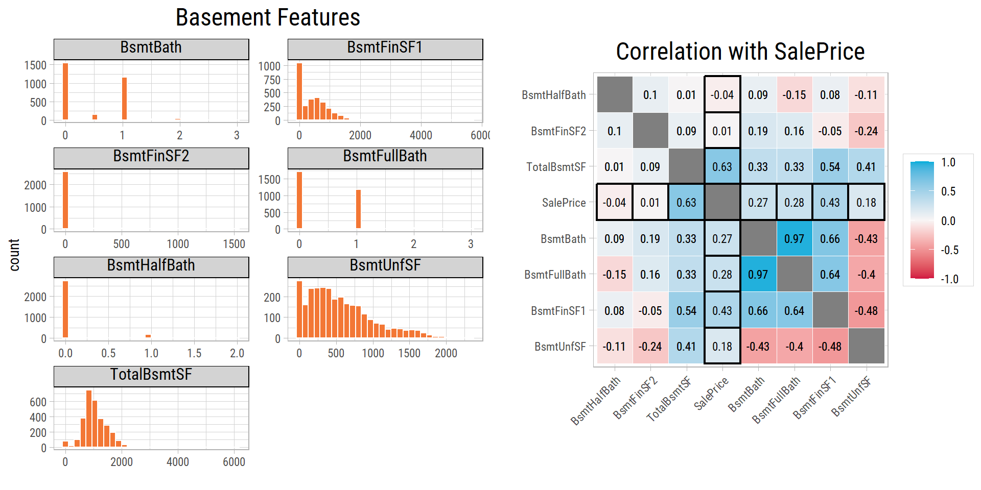
- Most properties have a basement.
- The column plots show that one category is much more common than the others in
BsmtFinType2and inBsmtCond.
vFeaturesChr <- dfBsmt %>% select(-SalePrice) %>% select_if(is.character) %>% colnames()

cowplot::plot_grid(plotlist = map(vFeaturesChr, ~ eda_plot_column(dfBsmt, .x)))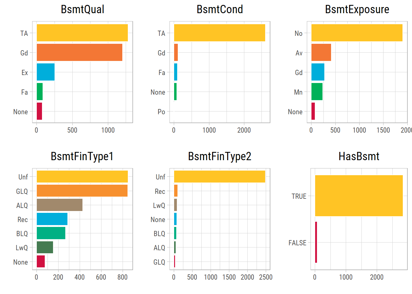
# cleanup
rm(dfBsmt, vFeaturesNum, vFeaturesChr)
Bathroom Features
- We create a new feature for the total number of bathrooms:
TotalBath=FullBath+ 0.5 *HalfBath+BsmtBath
# New features: HasFireplace
dfClean <- dfClean %>%
  mutate(TotalBath = FullBath + 0.5*HalfBath + BsmtBath)

dfBath <- dfClean %>% select(SalePrice, contains("Bath"))

vFeaturesNum <- dfBath %>% select(-SalePrice) %>% select_if(is.numeric) %>% colnames()

p1 <- eda_plot_histograms(dfBath, vFeaturesNum, plotTitle = "Bathroom Features")
p2 <- eda_plot_correlation_matrix(dfBath[c("SalePrice",vFeaturesNum)], outlineVar = "SalePrice", plotTitle = "Correlation with SalePrice")

cowplot::plot_grid(plotlist = list(p1, p2), ncol = 2)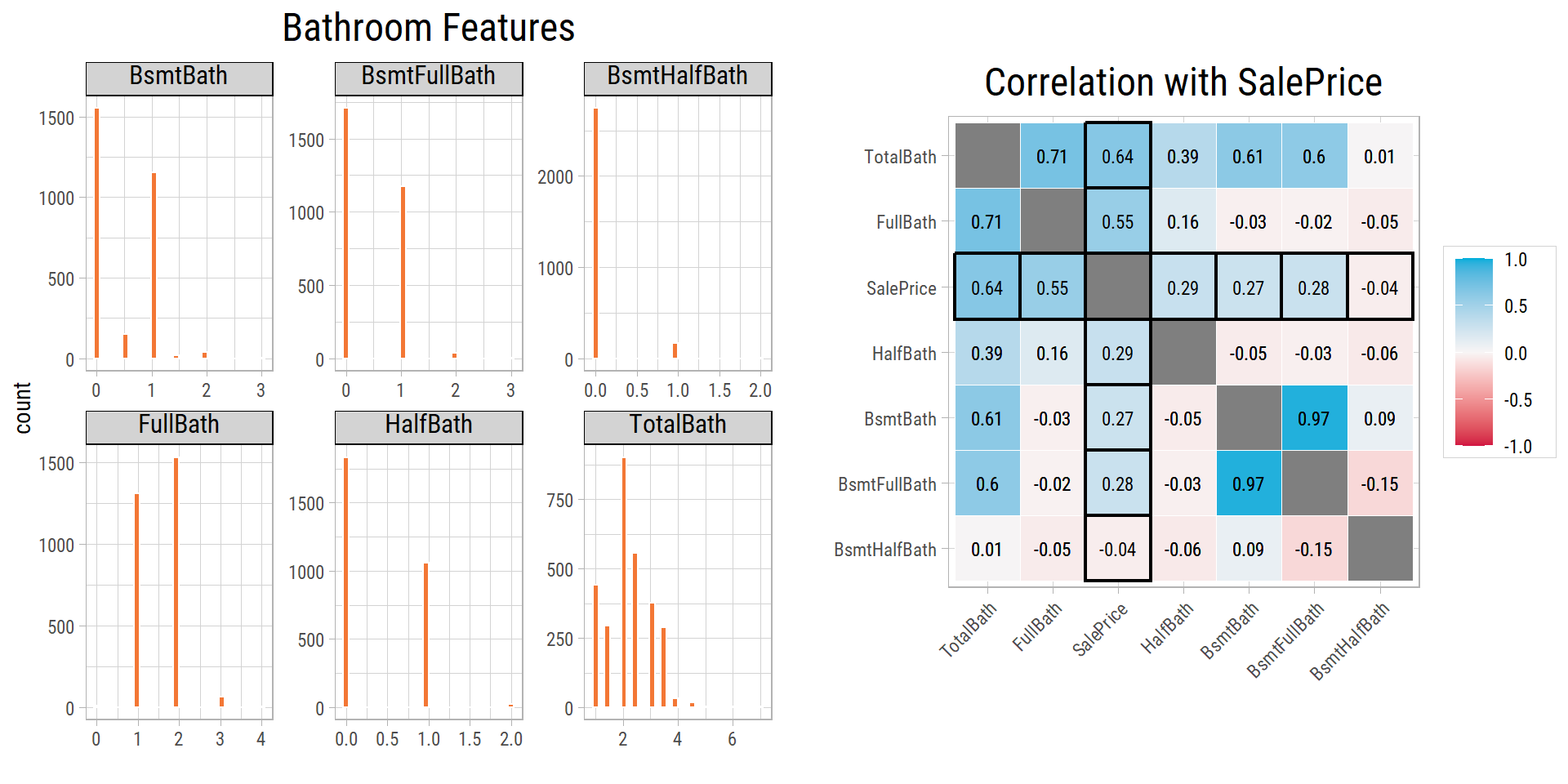
# cleanup
rm(dfBath, vFeaturesNum)
Fireplace Features
- 1420 properties have no fireplace. For these properties, we change
FireplaceQu(the fireplace quality) to None.
# 1. Change FireplaceQu to None if there is no fireplace
###############################################################################################################
dfClean %>% select(Id, Neighborhood, contains("Fire")) %>% dplyr::filter(Fireplaces == 0)
# A tibble: 1,420 × 4
Id Neighborhood Fireplaces FireplaceQu
<dbl> <chr> <dbl> <chr>
1 1 CollgCr 0 <NA>
2 6 Mitchel 0 <NA>
3 11 Sawyer 0 <NA>
4 13 Sawyer 0 <NA>
5 16 BrkSide 0 <NA>
6 18 Sawyer 0 <NA>
7 19 SawyerW 0 <NA>
8 20 NAmes 0 <NA>
9 27 NAmes 0 <NA>
10 30 BrkSide 0 <NA>
# ℹ 1,410 more rowsdfClean <- dfClean %>% mutate_at(vars("FireplaceQu"), ~ case_when(Fireplaces == 0 ~ "None", TRUE ~ .))- We create a new feature:
HasFireplace=Fireplaces> 0 - Many properties have a fireplace.
# New features: HasFireplace
dfClean <- dfClean %>%
  mutate(HasFireplace = (Fireplaces > 0),
         HasFireplace = as.character(HasFireplace))

dfFireplace <- dfClean %>% select(SalePrice, contains("Fireplace"))

vFeaturesNum <- dfFireplace %>% select(-SalePrice) %>% select_if(is.numeric) %>% colnames()
vFeaturesChr <- dfFireplace %>% select(-SalePrice) %>% select_if(is.character) %>% colnames()

p1 <- eda_plot_histograms(dfFireplace, vFeaturesNum, plotTitle = "Fireplace Features")
p2 <- cowplot::plot_grid(plotlist = map(vFeaturesChr, ~ eda_plot_column(dfFireplace, .x)))
p3 <- eda_plot_correlation_matrix(dfFireplace[c("SalePrice",vFeaturesNum)], outlineVar = "SalePrice", plotTitle = "Correlation with SalePrice")

grid.arrange(arrangeGrob(p1, p2, nrow = 2), p3, ncol = 2)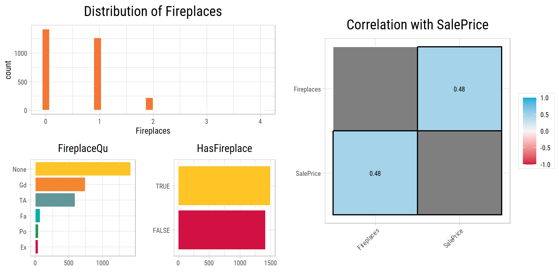
# cleanup
rm(dfFireplace, vFeaturesNum, vFeaturesChr)
Garage Features
If
GarageYrBltis missing, we set it toYearBuilt.157 properties have no garage. For these properties,
GarageType,GarageFinish,GarageQualandGarageCondare None.Garages are different in different neighborhoods. So we fill in each remaining missing value with the most common value (or the median value, for numbers) of the same
NeighborhoodandGarageType.
# 1. Change GarageYrBlt to YearBuilt if it is NA
############################################################################################################
dfClean <- dfClean %>% mutate(GarageYrBlt = if_else(is.na(GarageYrBlt), YearBuilt, GarageYrBlt))

# 2. Change NA values to None if there is no garage
############################################################################################################
dfClean %>% select(Id, Neighborhood, contains("Garage")) %>% dplyr::filter(GarageArea == 0)
# A tibble: 157 × 9
Id Neighborhood GarageType GarageYrBlt GarageFinish GarageCars GarageArea GarageQual GarageCond
<dbl> <chr> <chr> <dbl> <chr> <dbl> <dbl> <chr> <chr>
1 40 Edwards <NA> 1955 <NA> 0 0 <NA> <NA>
2 49 OldTown <NA> 1920 <NA> 0 0 <NA> <NA>
3 79 Sawyer <NA> 1968 <NA> 0 0 <NA> <NA>
4 89 IDOTRR <NA> 1915 <NA> 0 0 <NA> <NA>
5 90 CollgCr <NA> 1994 <NA> 0 0 <NA> <NA>
6 100 NAmes <NA> 1959 <NA> 0 0 <NA> <NA>
7 109 IDOTRR <NA> 1919 <NA> 0 0 <NA> <NA>
8 126 IDOTRR <NA> 1935 <NA> 0 0 <NA> <NA>
9 128 OldTown <NA> 1930 <NA> 0 0 <NA> <NA>
10 141 NAmes <NA> 1971 <NA> 0 0 <NA> <NA>
# ℹ 147 more rowsvFeaturesChr_garage <- dfClean %>% select(contains("Garage")) %>% select_if(is.character) %>% colnames()
dfClean <- dfClean %>% mutate_at(all_of(vFeaturesChr_garage), ~ case_when(GarageArea == 0 ~ "None", TRUE ~ .))
# 3. Change NA values in remaining features to the most common or median value in the Neighborhood for that GarageType
######################################################################################################################
dfClean %>% select(Id, Neighborhood, contains("Garage")) %>% dplyr::filter_all(any_vars(is.na(.)))# A tibble: 2 × 9
Id Neighborhood GarageType GarageYrBlt GarageFinish GarageCars GarageArea GarageQual GarageCond
<dbl> <chr> <chr> <dbl> <chr> <dbl> <dbl> <chr> <chr>
1 2127 OldTown Detchd 1910 <NA> 1 360 <NA> <NA>
2 2577 IDOTRR Detchd 1923 <NA> NA NA <NA> <NA> dfNeighborhood_mcv <- most_common_value_by_grouping(dfClean, c("Neighborhood","GarageType"), c("GarageQual","GarageFinish","GarageCond"))
dfNeighborhood_med <- median_by_grouping(dfClean, c("Neighborhood","GarageType"), c("GarageCars","GarageArea")) %>%
ungroup() %>%
mutate_if(is.numeric, as.integer)
dfClean <- dfClean %>%
mutate(GarageFinish = if_else(is.na(GarageFinish),
map2_chr(Neighborhood, GarageType, ~ with(dfNeighborhood_mcv, GarageFinish[Neighborhood==.x & GarageType==.y])),
GarageFinish)) %>%
mutate(GarageQual = if_else(is.na(GarageQual),
map2_chr(Neighborhood, GarageType, ~ with(dfNeighborhood_mcv, GarageQual[Neighborhood==.x & GarageType==.y])),
GarageQual)) %>%
mutate(GarageCond = if_else(is.na(GarageCond),
map2_chr(Neighborhood, GarageType, ~ with(dfNeighborhood_mcv, GarageCond[Neighborhood==.x & GarageType==.y])),
GarageCond)) %>%
mutate(GarageCars = if_else(is.na(GarageCars),
map2_dbl(Neighborhood, GarageType, ~ with(dfNeighborhood_med, GarageCars[Neighborhood==.x & GarageType==.y])),
GarageCars)) %>%
mutate(GarageArea = if_else(is.na(GarageArea),
map2_dbl(Neighborhood, GarageType, ~ with(dfNeighborhood_med, GarageArea[Neighborhood==.x & GarageType==.y])),
GarageArea))
# cleanup
rm(vFeaturesChr_garage, dfNeighborhood_mcv, dfNeighborhood_med)GarageAreaandGarageCarshave almost the same correlation withSalePrice.- We create a new feature:
HasGarage=GarageArea> 0 - Most properties have a garage.
- The column plots show that one category is much more common than the others in
GarageQualand inGarageCond.
# New features: HasGarage
dfClean <- dfClean %>%
  mutate(HasGarage = (GarageArea > 0),
         HasGarage = as.character(HasGarage))

dfGarage <- dfClean %>% select(SalePrice, contains("Garage"))

vFeaturesNum <- dfGarage %>% select(-SalePrice) %>% select_if(is.numeric) %>% colnames()
vFeaturesChr <- dfGarage %>% select(-SalePrice) %>% select_if(is.character) %>% colnames()

p1 <- eda_plot_histograms(dfGarage, vFeaturesNum, nCols = 2, plotTitle = "Garage Features")
p2 <- cowplot::plot_grid(plotlist = map(vFeaturesChr, ~ eda_plot_column(dfGarage, .x)))
p3 <- eda_plot_correlation_matrix(dfGarage[c("SalePrice",vFeaturesNum)], outlineVar = "SalePrice", plotTitle = "Correlation with SalePrice")

grid.arrange(arrangeGrob(p1, p2, nrow = 2), p3, ncol = 2)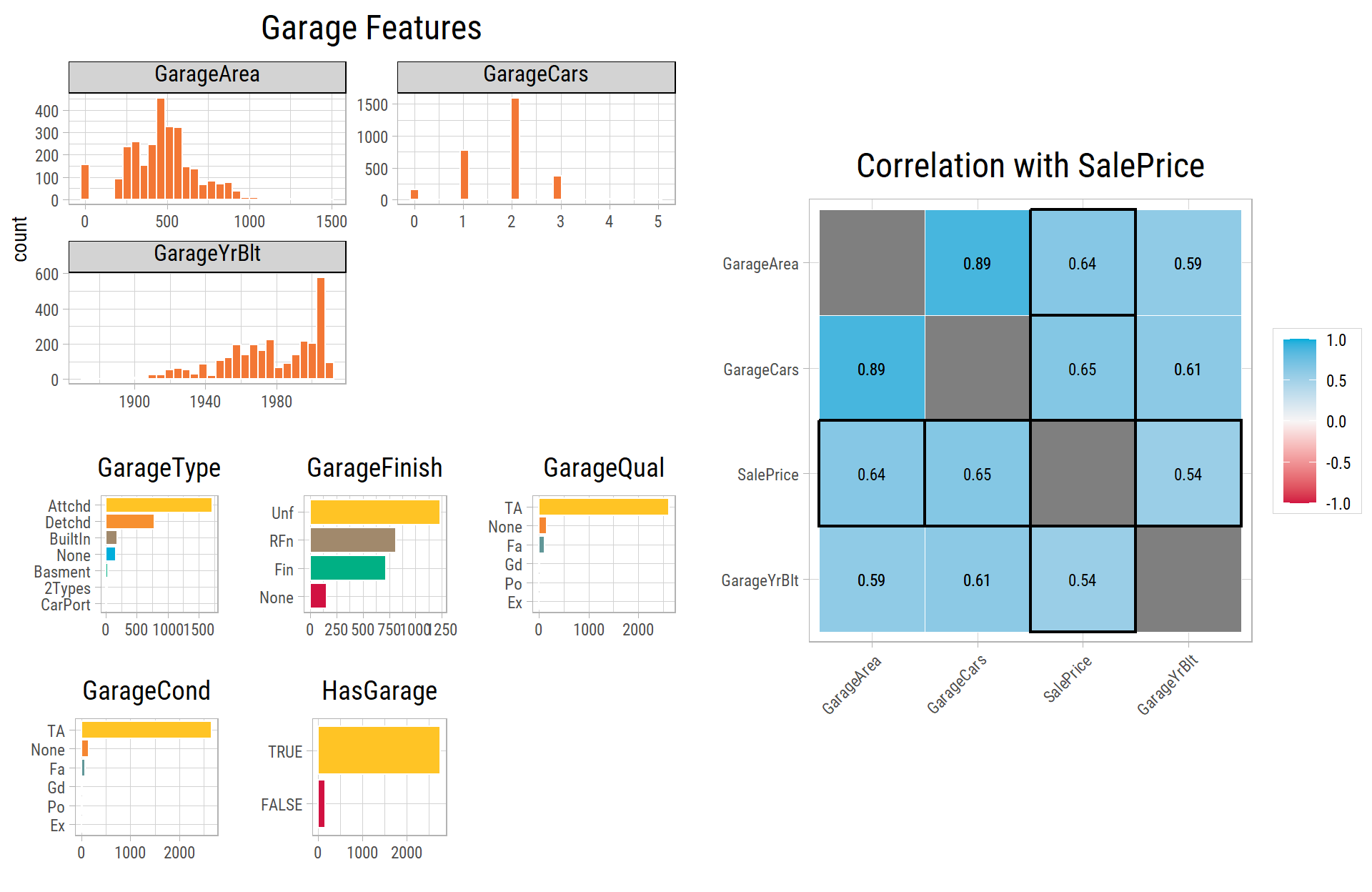
# cleanup
rm(dfGarage, vFeaturesNum, vFeaturesChr)
Masonry Features
For one property (
Id= 2611),MasVnrArea(the area of the masonry veneer) is 198, butMasVnrType(the type of masonry) is missing. We setMasVnrTypeto the most common type in the same neighborhood, among the properties that have masonry.We fill in the missing values of
MasVnrTypewith the most common values for the sameNeighborhoodandYearRemodAdd.We fill in the missing values of
MasVnrAreawith the median values for the sameNeighborhoodandMasVnrType. The median is the middle value: half the values are below it and half are above it.
# 1. Change MasVnrType in Id 2611 as the most common value in the Neighborhood
###############################################################################################################
dfClean %>% select(Id, Neighborhood, contains("Mas")) %>% dplyr::filter(Id == 2611)
# A tibble: 1 × 4
Id Neighborhood MasVnrType MasVnrArea
<dbl> <chr> <chr> <dbl>
1 2611 Mitchel <NA> 198masvnrtype_mcv <- dfClean %>% dplyr::filter(MasVnrArea > 0, Neighborhood == "Mitchel") %>%
most_common_value_by_grouping(c("Neighborhood"), "MasVnrType") %>% pull(MasVnrType)
dfClean <- dfClean %>% mutate(MasVnrType = if_else(Id == 2611, masvnrtype_mcv, MasVnrType))
# 2. Change remaining NA values in MasVnrType to most common values by Neighborhood and YearRemodAdd
###############################################################################################################
dfClean %>% select(Id, Neighborhood, contains("Mas")) %>% dplyr::filter_all(any_vars(is.na(.)))# A tibble: 23 × 4
Id Neighborhood MasVnrType MasVnrArea
<dbl> <chr> <chr> <dbl>
1 235 Gilbert <NA> NA
2 530 Crawfor <NA> NA
3 651 Somerst <NA> NA
4 937 SawyerW <NA> NA
5 974 Somerst <NA> NA
6 978 Somerst <NA> NA
7 1244 NridgHt <NA> NA
8 1279 CollgCr <NA> NA
9 1692 Gilbert <NA> NA
10 1707 Somerst <NA> NA
# ℹ 13 more rowsdfNeighborhood_mcv <- most_common_value_by_grouping(dfClean, c("Neighborhood","YearRemodAdd"), "MasVnrType") %>%
mutate(MasVnrType = if_else(is.na(MasVnrType), "None", MasVnrType))
dfClean <- dfClean %>%
mutate(MasVnrType = if_else(is.na(MasVnrType),
map2_chr(Neighborhood, YearRemodAdd, ~ with(dfNeighborhood_mcv, MasVnrType[Neighborhood == .x & YearRemodAdd == .y])),
MasVnrType))
# 3. Change NA values in MasVnrArea to median values by Neighborhood and MasVnrType
###############################################################################################################
dfClean %>% select(Id, Neighborhood, contains("Mas")) %>% dplyr::filter_all(any_vars(is.na(.)))# A tibble: 23 × 4
Id Neighborhood MasVnrType MasVnrArea
<dbl> <chr> <chr> <dbl>
1 235 Gilbert None NA
2 530 Crawfor None NA
3 651 Somerst None NA
4 937 SawyerW None NA
5 974 Somerst Stone NA
6 978 Somerst None NA
7 1244 NridgHt Stone NA
8 1279 CollgCr BrkFace NA
9 1692 Gilbert None NA
10 1707 Somerst Stone NA
# ℹ 13 more rowsdfNeighborhood_med <- median_by_grouping(dfClean, c("Neighborhood","MasVnrType"), "MasVnrArea")
dfClean <- dfClean %>%
mutate(MasVnrArea = if_else(is.na(MasVnrArea),
map2_dbl(Neighborhood, MasVnrType, ~ with(dfNeighborhood_med, MasVnrArea[Neighborhood == .x & MasVnrType == .y])),
MasVnrArea))
# cleanup
rm(masvnrtype_mcv, dfNeighborhood_mcv, dfNeighborhood_med)- We create a new feature:
HasMasVnr=MasVnrArea> 0 - Many properties have masonry.
# New features: HasMasVnr
dfClean <- dfClean %>%
  mutate(HasMasVnr = (MasVnrArea > 0),
         HasMasVnr = as.character(HasMasVnr))

dfMasVnr <- dfClean %>% select(SalePrice, contains("MasVnr"))

vFeaturesNum <- dfMasVnr %>% select(-SalePrice) %>% select_if(is.numeric) %>% colnames()
vFeaturesChr <- dfMasVnr %>% select(-SalePrice) %>% select_if(is.character) %>% colnames()

p1 <- eda_plot_histograms(dfMasVnr, vFeaturesNum, plotTitle = "Masonry Features")
p2 <- cowplot::plot_grid(plotlist = map(vFeaturesChr, ~ eda_plot_column(dfMasVnr, .x)))
p3 <- eda_plot_correlation_matrix(dfMasVnr[c("SalePrice",vFeaturesNum)], outlineVar = "SalePrice", plotTitle = "Correlation with SalePrice")

grid.arrange(arrangeGrob(p1, p2, nrow = 2), p3, ncol = 2)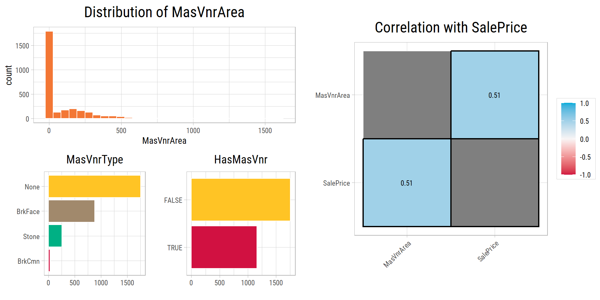
# cleanup
rm(dfMasVnr, vFeaturesNum, vFeaturesChr)
Pool Features
If the property has no pool, we change
PoolQC(the pool quality) to None.We fill in the remaining missing values of
PoolQCwith the most common value in the same neighborhood, among the properties that have a pool.
# 1. Change NA values in PoolQC to None if there is no pool
###############################################################################################################
dfClean %>% select(Id, Neighborhood, contains("Pool")) %>% dplyr::filter(PoolArea == 0)
# A tibble: 2,906 × 4
Id Neighborhood PoolArea PoolQC
<dbl> <chr> <dbl> <chr>
1 1 CollgCr 0 <NA>
2 2 Veenker 0 <NA>
3 3 CollgCr 0 <NA>
4 4 Crawfor 0 <NA>
5 5 NoRidge 0 <NA>
6 6 Mitchel 0 <NA>
7 7 Somerst 0 <NA>
8 8 NWAmes 0 <NA>
9 9 OldTown 0 <NA>
10 10 BrkSide 0 <NA>
# ℹ 2,896 more rowsdfClean <- dfClean %>% mutate(PoolQC = if_else(PoolArea == 0, "None", PoolQC))
# 2. Change NA values in remaining PoolQC to the most common value in the Neighborhood where PoolArea > 0
###############################################################################################################
(dfMissing <- dfClean %>% select(Id, Neighborhood, contains("Pool")) %>% dplyr::filter_all(any_vars(is.na(.))))# A tibble: 3 × 4
Id Neighborhood PoolArea PoolQC
<dbl> <chr> <dbl> <chr>
1 2421 NAmes 368 <NA>
2 2504 SawyerW 444 <NA>
3 2600 Mitchel 561 <NA> dfNeighborhood_mcv <- most_common_value_by_grouping(dfClean %>% dplyr::filter(PoolArea > 0), "Neighborhood", "PoolQC") %>%
mutate(PoolQC = if_else(is.na(PoolQC), "None", PoolQC))
dfMissing <- dfMissing %>% mutate(PoolQC = map_chr(Neighborhood, ~ with(dfNeighborhood_mcv, PoolQC[Neighborhood == .x])))
dfClean$PoolQC[dfClean$Id %in% dfMissing$Id] <- dfMissing$PoolQC
# cleanup
rm(dfNeighborhood_mcv, dfMissing)- We create a new feature:
HasPool=PoolArea> 0 - Most properties do not have a pool.
# New features: HasGarage
dfClean <- dfClean %>%
  mutate(HasPool = (PoolArea > 0),
         HasPool = as.character(HasPool))

dfPool <- dfClean %>% select(SalePrice, contains("Pool"))

vFeaturesNum <- dfPool %>% select(-SalePrice) %>% select_if(is.numeric) %>% colnames()
vFeaturesChr <- dfPool %>% select(-SalePrice) %>% select_if(is.character) %>% colnames()

p1 <- eda_plot_histograms(dfPool, vFeaturesNum, plotTitle = "Pool Features")
p2 <- cowplot::plot_grid(plotlist = map(vFeaturesChr, ~ eda_plot_column(dfPool, .x)))
p3 <- eda_plot_correlation_matrix(dfPool[c("SalePrice",vFeaturesNum)], outlineVar = "SalePrice", plotTitle = "Correlation with SalePrice")

grid.arrange(arrangeGrob(p1, p2, nrow = 2), p3, ncol = 2)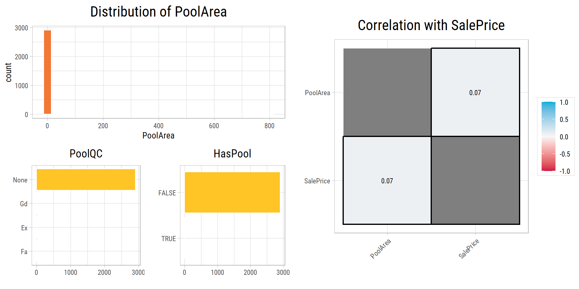
# cleanup
rm(dfPool, vFeaturesNum, vFeaturesChr)
Porch Features
- We create new features for:
- The total porch area:
PorchSF=OpenPorchSF+EnclosedPorch+3SsnPorch+ScreenPorch - Whether the property has a porch:
HasPorch=PorchSF> 0
- The total porch area:
# New features: PorchSF, HasPorch
dfClean <- dfClean %>%
  mutate(PorchSF = OpenPorchSF + EnclosedPorch + `3SsnPorch` + ScreenPorch) %>%
  mutate(HasPorch = PorchSF > 0,
         HasPorch = as.character(HasPorch))

dfPorch <- dfClean %>% select(SalePrice, contains("Porch"))

vFeaturesNum <- dfPorch %>% select(-SalePrice) %>% select_if(is.numeric) %>% colnames()
vFeaturesChr <- dfPorch %>% select(-SalePrice) %>% select_if(is.character) %>% colnames()

p1 <- eda_plot_histograms(dfPorch, vFeaturesNum, plotTitle = "Porch Features")
p2 <- cowplot::plot_grid(plotlist = map(vFeaturesChr, ~ eda_plot_column(dfPorch, .x)))
p3 <- eda_plot_correlation_matrix(dfPorch[c("SalePrice",vFeaturesNum)], outlineVar = "SalePrice", plotTitle = "Correlation with SalePrice")

grid.arrange(arrangeGrob(p1, p2, nrow = 2), p3, ncol = 2)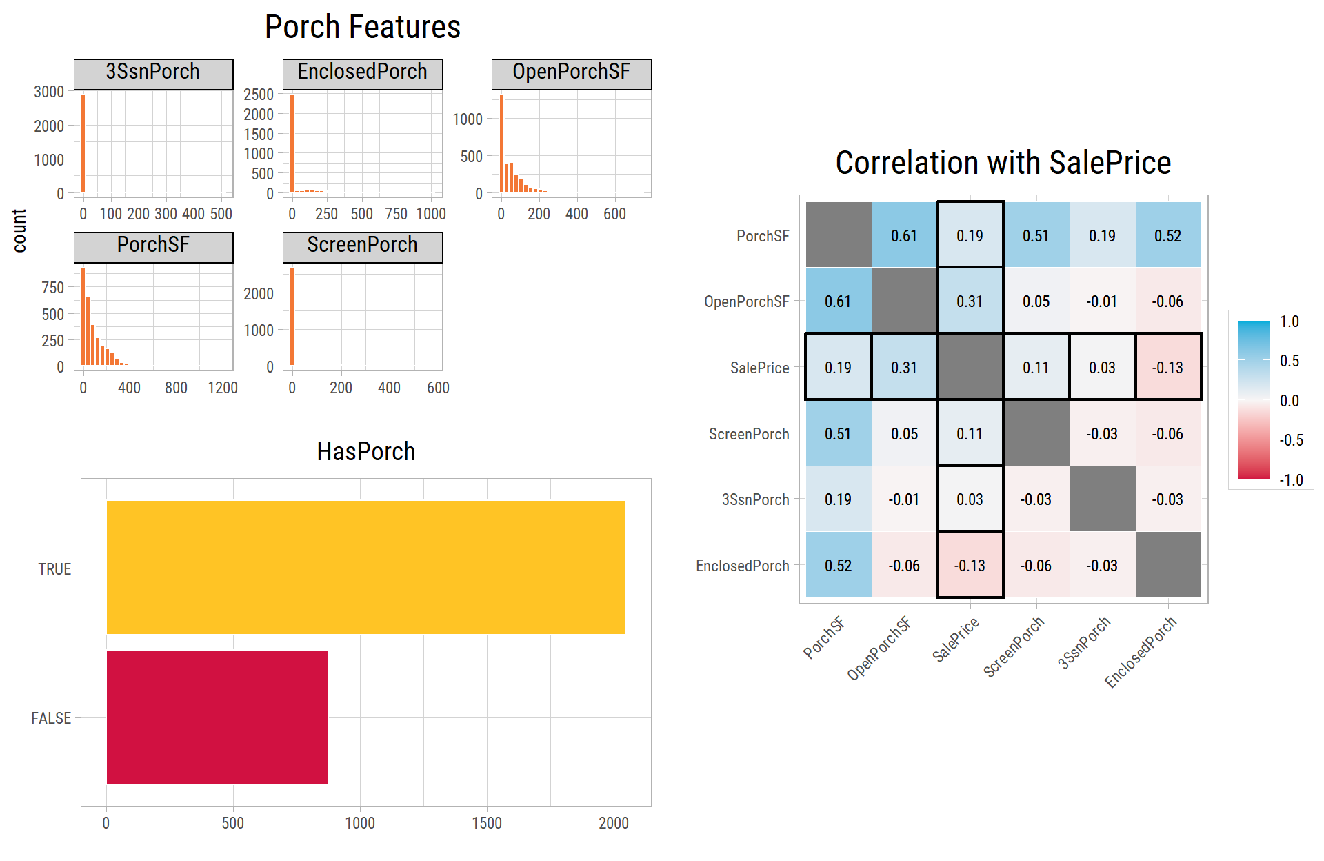
# cleanup
rm(dfPorch, vFeaturesNum, vFeaturesChr)
Built Area Features
- We create a new feature for the total built area in square feet:
TotalSF=GrLivArea+TotalBsmtSF
dfClean <- dfClean %>%
  mutate(TotalSF = GrLivArea + TotalBsmtSF)

vFeaturesNum <- c("TotalSF","GrLivArea","TotalBsmtSF")

p1 <- eda_plot_histograms(dfClean, vFeaturesNum, plotTitle = "Built Area Features")
p2 <- eda_plot_correlation_matrix(dfClean[c("SalePrice",vFeaturesNum)], outlineVar = "SalePrice", plotTitle = "Correlation with SalePrice")

cowplot::plot_grid(plotlist = list(p1, p2), ncol = 2)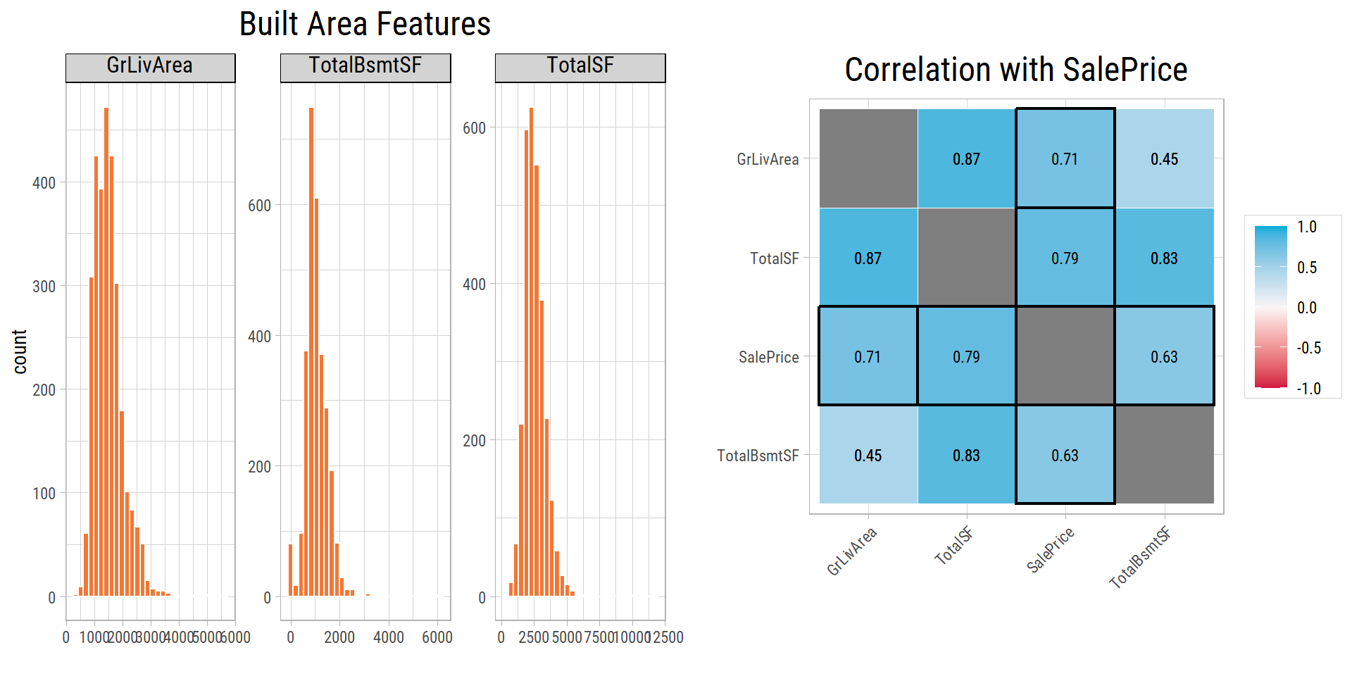
# cleanup
rm(vFeaturesNum)
Construction Year Features
- We create new features for:
- The period when the property was built (
Vintage): 1945 or earlier, 1946-1999, 2000 or later - The age of the property when it was sold, counted from its last remodel (or from its construction, if it was never remodeled):
PropertyAge=YrSold-YearRemodAdd - Whether the property was new or newly remodeled when it was sold:
IsNew=YearRemodAdd==YrSold - Whether the property was ever remodeled:
IsRemod=YearRemodAdd>YearBuilt
- The period when the property was built (
# New feature: Vintage
dfClean <- dfClean %>%
  mutate(Vintage = cut(YearBuilt, breaks = c(1800, 1945, 1999, 2100),
                       labels = c("1945 or ealier","1946-1999","2000 or later"),
                       ordered_result = T)) %>%
  mutate(PropertyAge = YrSold - YearRemodAdd) %>%
  mutate(IsNew = (YearBuilt == YrSold),
         IsNew = as.character(IsNew)) %>%
  mutate(IsRemod = (YearRemodAdd > YearBuilt),
         IsRemod = as.character(IsRemod))

vFeaturesNum <- dfClean %>% select(contains("Year"),contains("Yr"),"PropertyAge") %>% colnames() %>% sort()
vFeaturesChr <- c("IsNew","IsRemod","Vintage")

p1 <- eda_plot_histograms(dfClean, vFeaturesNum, nCols = 2, plotTitle = "Construction Year Features")
p2 <- cowplot::plot_grid(plotlist = map(vFeaturesChr, ~ eda_plot_column(dfClean, .x)))
p3 <- eda_plot_correlation_matrix(dfClean[c("SalePrice",vFeaturesNum)], outlineVar = "SalePrice", plotTitle = "Correlation with SalePrice")

grid.arrange(arrangeGrob(p1, p2, nrow = 2), p3, ncol = 2)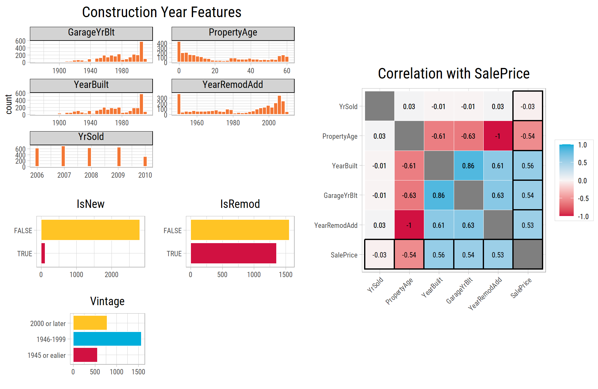
# cleanup
rm(vFeaturesNum, vFeaturesChr)
Neighborhood Features
Type of Neighborhood: The dataset has 25 neighborhoods. In real estate, location is very important. Some neighborhoods clearly have higher prices than others.
We can put the neighborhoods into fewer groups, by their median SalePrice:
- Type1: StoneBr, NridgHt, NoRidge
- Type2: Veenker, Timber, Somerst
- Type3: Crawfor, CollgCr, ClearCr, Blmngtn, Gilbert, NWAmes, SawyerW
- Type4: Mitchel, NPkVill, NAmes, SWISU, Sawyer, Blueste, BrkSide, Edwards, OldTown
- Type5: IDOTRR, BrDale, MeadowV
dfClean <- dfClean %>%
  # lNeighborhoodTypes is defined with the neighborhood map at the start of this post
  mutate(NeighborhoodType = fct_collapse(Neighborhood, !!!lNeighborhoodTypes)) %>%
  mutate(NeighborhoodType = factor(NeighborhoodType, levels = c("Type5","Type4","Type3","Type2","Type1"), ordered = TRUE))

p1 <- eda_plot_box(dfClean, "Neighborhood", "SalePrice", yLabelsScale = scales::label_dollar(accuracy = 1))
p2 <- eda_plot_box(dfClean, "NeighborhoodType", "SalePrice", yLabelsScale = scales::label_dollar(accuracy = 1))

cowplot::plot_grid(plotlist = list(p1, p2), ncol = 2)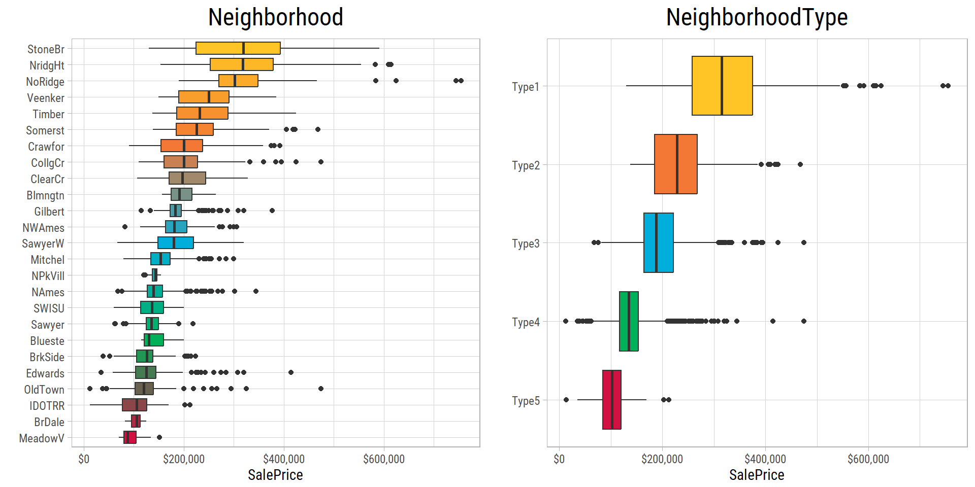
Other Missing Features
In
MiscFeature,AlleyandFence, we change the missing values to None.In
Utilities,FunctionalandSaleType, we fill in the missing values with the most common value of each feature.In
LotFrontage, we fill in the missing values with the median value of the sameNeighborhood.In
MSZoning,KitchenQual,Exterior1st,Exterior2ndandElectrical, we fill in the missing values with the most common value of the sameNeighborhood.
# 1. & 2. change NA values to None or most common value of that feature
####################################################################################################################
dfClean <- dfClean %>%
  mutate_at(c("MiscFeature", "Alley", "Fence"), change_na_to, value = "None") %>%
  mutate_at(c("Utilities"), change_na_to_most_common_value) %>%
  mutate_at(c("Functional"), change_na_to_most_common_value) %>%
  mutate_at(c("SaleType"), change_na_to_most_common_value)

# 3. In LotFrontage, change NA values to the median value by neighborhood
####################################################################################################################
dfNeighborhood_med <- median_by_grouping(dfClean, "Neighborhood", "LotFrontage")

dfClean <- dfClean %>%
  mutate(LotFrontage = if_else(is.na(LotFrontage),
                               map_dbl(Neighborhood, ~ with(dfNeighborhood_med, LotFrontage[Neighborhood == .x])),
                               LotFrontage))

# 4. In MSZoning,KitchenQual,Exterior1st,Exterior2nd,Electrical change NA values to the median value by neighborhood
dfNeighborhood_mcv <- most_common_value_by_grouping(dfClean, "Neighborhood", c("MSZoning","KitchenQual","Exterior1st","Exterior2nd","Electrical"))

dfClean <- dfClean %>%
  mutate(MSZoning = if_else(is.na(MSZoning),
                            map_chr(Neighborhood, ~ with(dfNeighborhood_mcv, MSZoning[Neighborhood == .x])),
                            MSZoning)) %>%
  mutate(KitchenQual = if_else(is.na(KitchenQual),
                              map_chr(Neighborhood, ~ with(dfNeighborhood_mcv, KitchenQual[Neighborhood == .x])),
                              KitchenQual)) %>%
  mutate(Exterior1st = if_else(is.na(Exterior1st),
                              map_chr(Neighborhood, ~ with(dfNeighborhood_mcv, Exterior1st[Neighborhood == .x])),
                              Exterior1st)) %>%
  mutate(Exterior2nd = if_else(is.na(Exterior2nd),
                              map_chr(Neighborhood, ~ with(dfNeighborhood_mcv, Exterior2nd[Neighborhood == .x])),
                              Exterior2nd)) %>%
  mutate(Electrical = if_else(is.na(Electrical),
                              map_chr(Neighborhood, ~ with(dfNeighborhood_mcv, Electrical[Neighborhood == .x])),
                              Electrical))

# cleanup
rm(dfNeighborhood_med, dfNeighborhood_mcv)
Label Encoding
The data description shows that the categories of many features have a natural order. These features are called ordinal features:
LotShape: Reg, IR1, IR2, IR3LandSlope: Gtl, Mod, SevExterQual: Ex, Gd, TA, Fa, PoExterCond: Ex, Gd, TA, Fa, PoBsmtQual: Ex, Gd, TA, Fa, Po, NoneBsmtCond: Ex, Gd, TA, Fa, Po, NoneBsmtExposure: Gd, Av, Mn, No, NoneBsmtFinType1: GLQ, ALQ, BLQ, Rec, LwQ, Unf, NoneBsmtFinType2: GLQ, ALQ, BLQ, Rec, LwQ, Unf, NoneHeatingQC: Ex, Gd, TA, Fa, PoCentralAir: Y, NKitchenQual: Ex, Gd, TA, Fa, PoFunctional: Typ, Min1, Min2, Mod, Maj1, Maj2, Sev, SalFireplaceQu: Ex, Gd, TA, Fa, Po, NoneGarageFinish: Fin, RFn, Unf, NoneGarageQual: Ex, Gd, TA, Fa, Po, NoneGarageCond: Ex, Gd, TA, Fa, Po, NoneStreet: Grvl, PavePavedDrive: Y, P, N
Most of these features use the same order: Ex (excellent), Gd (good), TA (typical/average), Fa (fair), Po (poor). Some of them also have the category None. So we can give these features one common set of ordered categories: Ex, Gd, TA, Fa, Po, None.
Two features already use numbers for their order:
OverallQual: 10 to 1OverallCond: 10 to 1
MoSold (the month of the sale) repeats in a cycle every year, so we treat it as a category, not as a number.
YrSold has only 5 values, from 2006 to 2010, so we also treat it as a category.
In categorical features where several categories have fewer than 10 properties, we put these rare categories together in one category named Other.
is.nominal <- function(Z) {
  return(is.factor(Z) & !is.ordered(Z))
}

dfClean <- dfClean %>%
  mutate(MoSold = as.factor(MoSold)) %>%
  mutate(YrSold = as.factor(YrSold)) %>%
  mutate(MSSubClass = as.character(MSSubClass)) %>%
  mutate_at(c("ExterCond","ExterQual","BsmtQual","BsmtCond","HeatingQC","KitchenQual","FireplaceQu","GarageQual","GarageCond"),
            factor, levels = c("Ex","Gd","TA","Fa","Po","None"), ordered = TRUE) %>%
  mutate_at(c("BsmtFinType1","BsmtFinType2"),
            factor, levels = c("GLQ", "ALQ", "BLQ", "Rec", "LwQ", "Unf", "None"), ordered = TRUE) %>%
  mutate(LotShape = factor(LotShape, levels = c("Reg","IR1","IR2","IR3"), ordered = TRUE)) %>%
  mutate(LandSlope = factor(LandSlope, levels = c("Gtl", "Mod", "Sev"), ordered = TRUE)) %>%
  mutate(BsmtExposure = factor(BsmtExposure, levels = c("Gd", "Av", "Mn", "No", "None"), ordered = TRUE)) %>%
  mutate(Functional = factor(Functional, levels = c("Typ", "Min1", "Min2", "Mod", "Maj1", "Maj2", "Sev", "Sal"), ordered = TRUE)) %>%
  mutate(GarageFinish = factor(GarageFinish, levels = c("Fin", "RFn", "Unf", "None"), ordered = TRUE)) %>%
  mutate(Street = factor(Street, levels = c("Pave","Grvl"), ordered = TRUE)) %>%
  mutate(PavedDrive = factor(PavedDrive, levels = c("Y","P","N"), ordered = TRUE)) %>%
  mutate(OverallCond = ordered(OverallCond, levels = 1:10),
         OverallQual = ordered(OverallQual, levels = 1:10)) %>%
  mutate(CentralAir = ordered(CentralAir, levels = c("Y","N")),
         HasGarage = ordered(HasGarage, levels = c("TRUE", "FALSE")),
         HasFireplace = ordered(HasFireplace, levels = c("TRUE", "FALSE")),
         HasMasVnr = ordered(HasMasVnr, levels = c("TRUE", "FALSE")),
         HasPorch = ordered(HasPorch, levels = c("TRUE", "FALSE")),
         IsNew = ordered(IsNew, levels = c("TRUE","FALSE")),
         IsRemod = ordered(IsRemod, levels = c("TRUE","FALSE"))) %>%
  # mutate_if(is.ordered, fct_rev) %>% # reverse the factor levels before assigning an integer order
  # mutate_if(is.ordered, function(Z) as.integer(Z) - 1) %>%
  mutate_if(is.character, as.factor) %>%
  mutate_if(is.nominal, ~ fct_lump_min(.x, min = 10)) %>%
  mutate_if(is.logical, as.factor)
Features to Drop
Highly Correlated Features
We drop some features from the rest of the analysis, because they are strongly correlated with other features, or because a similar new feature replaces them.
(vFeatures_to_exclude <- c("BsmtFullBath","GarageCars","GarageYrBlt",
                           "GrLivArea","PoolArea",
                           "YearBuilt","YearRemodAdd","Neighborhood",
                           "OpenPorchSF","EnclosedPorch","3SsnPorch","ScreenPorch"))
[1] "BsmtFullBath" "GarageCars" "GarageYrBlt" "GrLivArea" "PoolArea" "YearBuilt" "YearRemodAdd" "Neighborhood" "OpenPorchSF"
[10] "EnclosedPorch" "3SsnPorch" "ScreenPorch" Let’s check these choices. For every pair of features, we measure their association, which tells how strongly the two features are related. We use a measure that suits each type of pair: the Pearson correlation for two numerical features, Cramer’s V for two categorical features, and the correlation ratio for one numerical and one categorical feature. All these measures are near 0 when there is no relationship. Features with many categories can seem related to everything by chance, so Cramer’s V and the correlation ratio include a correction (bias correction) for this.
mAssoc <- association_matrix(dfClean %>% select(-Id))

# one row per pair of features, strongest association first
mUpper <- which(upper.tri(mAssoc), arr.ind = T)
dfAssocPairs <- tibble(feature1 = rownames(mAssoc)[mUpper[, 1]],
                       feature2 = colnames(mAssoc)[mUpper[, 2]],
                       association = mAssoc[mUpper],
                       measure = attr(mAssoc, "measure")[mUpper]) %>%
  drop_na(association) %>%
  arrange(desc(abs(association)))

assoc_of <- function(f1, f2) {
  dfAssocPairs %>%
    filter((feature1 == f1 & feature2 == f2) | (feature1 == f2 & feature2 == f1)) %>%
    pull(association) %>%
    round(2)
}

vFeaturesAssoc <- dfAssocPairs %>% filter(abs(association) >= 0.85) %>% select(feature1, feature2) %>% unlist() %>% unique()
vPorchAssoc <- map_dbl(c("OpenPorchSF","EnclosedPorch","3SsnPorch","ScreenPorch"), ~ assoc_of(.x, "PorchSF"))
Here are the 36 features that have an association of 0.85 or more with at least one other feature. Related features are next to each other:
eda_plot_association_matrix(dfClean[vFeaturesAssoc], plotTitle = "Features with an association of 0.85 or more with another feature")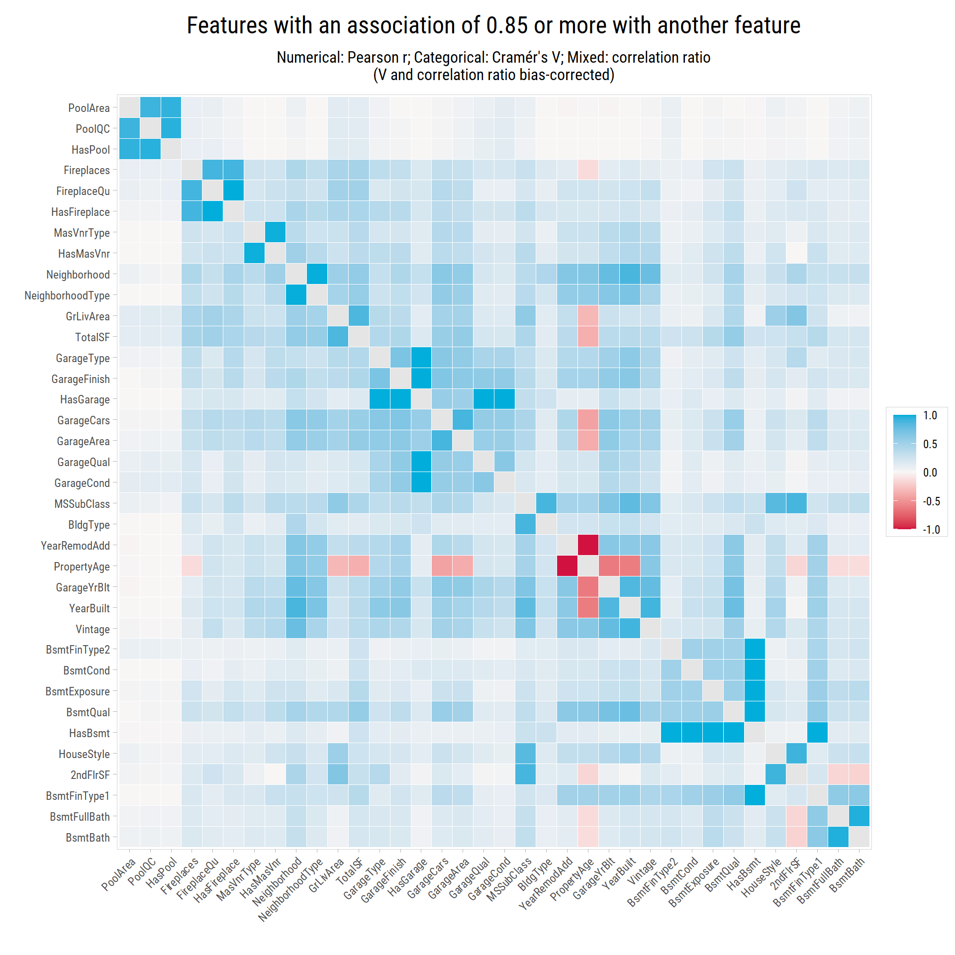
- Most of the features that we drop have a strong association with another feature:
GarageCarswithGarageArea(0.89),GrLivAreawithTotalSF(0.87),BsmtFullBathwithBsmtBath(0.97),PoolAreawithHasPool(0.94),YearBuiltwithVintage(0.9),GarageYrBltwithYearBuilt(0.86),YearRemodAddwithPropertyAge(-1), andNeighborhoodwithNeighborhoodType(1). - The four porch features have only a medium association with
PorchSF(between 0.19 and 0.61). So they do not repeat its information. We drop them becausePorchSF, their total area, replaces them. - The matrix also finds features that repeat information, which we have not dropped yet.
HasGarage,HasFireplaceandHasMasVnrgive the same information as the None category of the garage, fireplace and masonry features (Cramer’s V of about 1). Also,MSSubClasshas a strong association withBldgType(0.89) and withHouseStyle(0.83). Models that use decision trees are not affected by such repeated information. But in linear models, features that repeat each other (collinear features) make the results unreliable. So we will remove them before we build the models in Part 3.
Skewed Categorical Features
If more than 95% of the properties have the same category in a feature, the feature probably does not help to predict the price. An extreme example is Utilities, which has only 2 categories in the dataset: AllPub and NoSeWa. Only 1 property has NoSeWa, and all the others have AllPub. So features like this one do not help to predict the price.
For each categorical feature, let’s look at the share of its most common category. Let’s also count its rare categories, which have fewer than 10 properties:
p_dominance <- eda_plot_category_dominance(dfClean, threshold = 0.95, minCount = 10)
p_dominance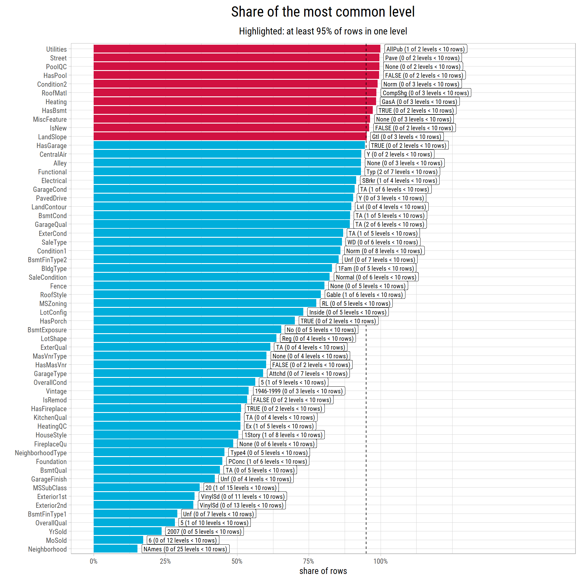
dfDominance <- p_dominance$data
dfRare <- dfDominance %>% filter(share < 0.95, n_rare > 0) %>% arrange(desc(n_rare), desc(share))- 11 features are above the 95% line, so we drop them. The plots below show them.
- Of the other features, 13 have at least one rare category with fewer than 10 properties, such as Functional, GarageQual, Electrical. For a model, each category becomes a separate feature with the values 0 and 1 (a dummy variable). A dummy variable for a rare category has only a few properties, so the model cannot measure its effect reliably. One way to solve this problem is to put the rare categories together in one category.
vFeatures_skewed <- dfClean %>%
  select_if(is.factor) %>%
  gather(feature, value) %>%
  group_by(feature, value) %>%
  count() %>%
  mutate(perc = n/nrow(dfClean)) %>%
  dplyr::filter(perc > 0.95) %>%
  pull(feature)

cowplot::plot_grid(plotlist = map(vFeatures_skewed, ~ eda_plot_column(dfClean, .x)))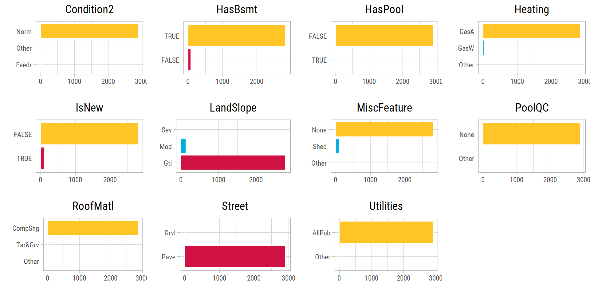
# Features to exclude for modelling
vFeatures_to_exclude <- c(vFeatures_to_exclude, vFeatures_skewed) %>% unique()

# cleanup
rm(vFeatures_skewed)
Finalized Data
# print("Following features are dropped")
# print(vFeatures_to_exclude)

# Finalized dataset
dfClean <- dfClean %>% select(-one_of(vFeatures_to_exclude))

# determine the numerical features
vFeaturesNum <- dfClean %>% select(-Id) %>% select_if(is.numeric) %>% colnames() %>% sort()

# determine the categorical features
vFeaturesCat <- dfClean %>% select(-Id) %>% select_if(is.factor) %>% colnames() %>% sort()
# vFeaturesCat1 <- vFeaturesCat[map_int(vFeaturesCat, ~ length(levels(dfClean[[.x]]))) > 5]
vFeaturesCat1 <- dfClean %>% select_if(is.ordered) %>% colnames() %>% sort()
vFeaturesCat2 <- setdiff(vFeaturesCat, vFeaturesCat1)

print("Dimensions of the finalized dataset")
[1] "Dimensions of the finalized dataset"dim(dfClean)[1] 2919 73print(glue::glue("Excluding Id, there are {(ncol(dfClean)-1)} features in the finalized dataset."))Excluding Id, there are 72 features in the finalized dataset.print(glue::glue("There are {length(vFeaturesNum)} numerical, {length(vFeaturesCat1)} ordinal and {length(vFeaturesCat2)} nominal features."))There are 26 numerical, 26 ordinal and 20 nominal features.The finalized dataset has 2919 properties and 73 columns: the Id and 72 features, including SalePrice. We save it, so that the next posts can use it:
# cache = FALSE: always save the current data. Part 3 checks the contents of this file (not its date), so saving
# the same data again does not make Part 3 tune its models again.
save(dfClean, vTestIDs, vFeaturesNum, vFeaturesCat, vFeaturesCat1, vFeaturesCat2, vFeatures_to_exclude,
     file = "Ames_Housing_Clean.Rda")
Next Steps
The data is now clean and ready. In Part 2, we explore this dataset, one feature at a time, then two and three features at a time, to find which features affect the sale price.