Ames Housing - Part 3 - Closing the deal - Building Models
Other posts in this series:
- Ames Housing - Part 1 - Laying the foundation - Building a Data Pipeline
- Ames Housing - Part 2 - Walkthrough - An Exploratory Data Analysis
In Part 1, we built a data pipeline that cleans the Ames Housing dataset, and in Part 2, we explored the finalized dataset.
In this post, we build linear and non-linear models, and we find out how well they predict the SalePrice of properties. A model is a formula that a computer learns from examples. A linear model adds up the features, each multiplied by a number (a coefficient) that it learns from the data. A non-linear model can also learn curved relationships.
Evaluation Criteria
To measure how good a model is, we use the root mean squared error (RMSE) between the log of the predicted price and the log of the actual SalePrice. RMSE is the typical size of a prediction error, so a lower RMSE is better. We use the log of the prices so that an error of 10% counts the same for an expensive house and for a cheap house.
Steps for Building Models
Each model has settings that it cannot learn from the data. We must choose them before training. These settings are called hyperparameters. To choose the best hyperparameters, we use K-fold cross validation, as described in the steps below:
- Remove features that repeat the information of other features, and change ordinal features into scores.
- Split the training data into K parts (folds). Each time, the model learns from all the folds except one (the training part), and we check its predictions on the remaining fold (the validation part). We split the data in a way that keeps a similar mix of prices in each fold (stratified sampling).
- Choose the linear and non-linear models to use.
- For each model, make a set (a grid) of hyperparameter combinations that covers the possible values evenly (a space-filling grid).
- For each combination, train the model on the training part and make predictions on the validation part. Repeat this for all the folds.
- Calculate the RMSE, and choose the combination with the lowest RMSE.
- Train each model again, with its best combination, on the complete training set.
- Calculate the RMSE of each final model on the testing set, which has properties that the models have not seen.
- Choose the model with the lowest RMSE.
Removing Collinear Predictors
Many features in this dataset describe the same thing in different ways. Also, some of the features that we created in Part 1 repeat others. A model cannot use categories directly, so each category becomes a separate feature with the values 0 and 1 (a dummy variable). After this change, some features are exact combinations of other features (we call them collinear). A linear model cannot separate the effects of collinear features. So its coefficients become unreliable, or it cannot calculate them at all, and lm (the basic linear model in R) gives a warning about a “rank-deficient fit”. Models that use decision trees are not affected by repeated information. But if we remove it, the linear models work correctly and all the models are simpler.
The association matrix in Part 1 showed which features repeat each other. We drop these features, because other features already give their information:
HasGarage,HasFireplaceandHasMasVnrare the same as, or almost the same as, the None category ofGarageType,FireplaceQuandMasVnrType.MSSubClasscombines the type and the style of a building.BldgTypeandHouseStylealready give this information. Its duplex category is identical to the duplex category ofBldgType.TotalBathis exactlyFullBath + 0.5 * HalfBath + BsmtBath. We dropHalfBath, notTotalBath. So we keep the total, which is one of the most important features for the decision tree models. And we lose no information, because we can calculateHalfBathfrom the other three features.
Encoding Ordinal Features
The categories of features such as OverallQual or KitchenQual have a natural order. These are ordinal features. By default, step_dummy() changes an ordinal feature into several features called polynomial contrasts. It makes one new feature for each category except one, and these features describe straight, curved and more complex trends across the grades. But some grades are very rare. For example, only one property has an OverallCond of 1. So a rare grade can be missing from a fold. Then some of these new features become collinear in that fold.
Instead, we change each ordinal feature into one whole number (a score) that follows the order of its categories: 1, 2, 3 and so on. This assumes that the steps between the grades are equal. First, we drop the categories that no property has, such as a Poor exterior quality, so that the scores have no gaps. Here are the results of a linear model with each method, on the same folds:
dfEncodingComparison %>%
  mutate(lm_cv_rmse = round(lm_cv_rmse, 4)) %>%
knitr::kable(col.names = c("Encoding of ordinal features", "Predictors", "Folds with a rank-deficient fit", "lm cross validated RMSE"))| Encoding of ordinal features | Predictors | Folds with a rank-deficient fit | lm cross validated RMSE |
|---|---|---|---|
| polynomial contrasts | 214 | 4 | 0.1470 |
| ordinal scores | 151 | 0 | 0.1336 |
encoding_value <- function(encodingName, column) dfEncodingComparison[[column]][dfEncodingComparison$encoding == encodingName]- With polynomial contrasts,
lmcannot calculate all the coefficients in 4 of the 5 folds. With scores, this problem happens in 0 folds. - With scores, the number of features goes down from 214 to 151, and the cross validated RMSE of
lmgoes down from 0.147 to 0.134. The simpler method works better on new data, because the model does not have to learn a separate effect for each rare grade.
Finally, step_lincomb() checks whether any features are still exact combinations of other features. This could happen because properties without a basement or a garage have the None category in every basement or garage feature. With scores, it finds no such features.
After these steps, there are 151 features, and a linear model can calculate a coefficient for each of them:
model_lm_check <- lm(target ~ ., data = dfTrain_Proc %>% select(-Id))
print(glue::glue("{sum(is.na(coef(model_lm_check)))} of {length(coef(model_lm_check))} coefficients could not be estimated"))
0 of 152 coefficients could not be estimatedPartitioning Training Data
We split the training data into 5 folds. In each fold, the model learns from 80% of the data, and we compare its predictions with the actual prices on the other 20%.
Let’s look at the spread (distribution) of the target, which is the value that we want to predict, in all the folds:
cv_folds %>%
  mutate(target = map(splits, function(Z) bind_rows(training(Z) %>% select(target) %>% mutate(type = "training"),
                                                    testing(Z) %>% select(target) %>% mutate(type = "validation")))) %>%
  select(-splits) %>%
  unnest(cols = c(target)) %>%
  ggplot(aes(x = target)) +
  geom_histogram(bins = 30, color = "white", fill = "#F37735") +
  labs(x = "log(SalePrice)") +
  facet_grid(type ~ id)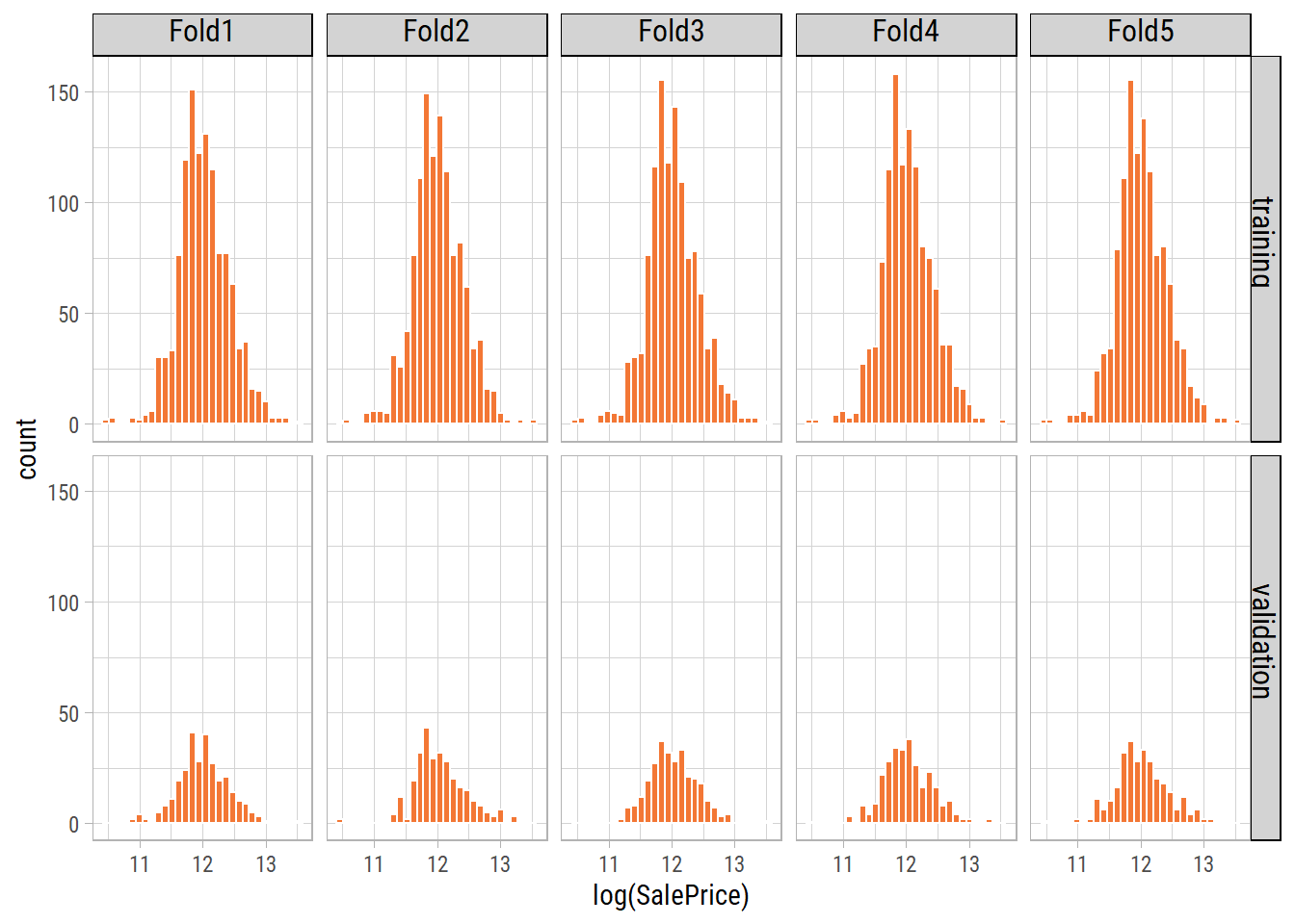
Because we use stratified sampling, the prices have similar distributions in the training part and in the validation part of each fold.
Linear Models
Ordinary Least Squares Regression
First, we use cross validation to test a simple linear model on the training data. This model, called ordinary least squares, finds the straight-line formula with the smallest squared errors. Its result is our starting point (benchmark). If more complex models are not much better than this result, they are not worth the extra effort.
model_spec_lmLinear Regression Model Specification (regression)
Computational engine: lm cv_results_lm# A tibble: 1 × 1
mean_rmse
<dbl>
1 0.134rmse_val <- cv_results_lm %>% pull(mean_rmse)What’s notable?
- A linear model with all the features gives an RMSE of 0.1336.
- This is the simplest and fastest model, and it has no hyperparameters to choose.
A residual is the difference between the actual value and the predicted value, here of log(SalePrice). Residual plots show if the errors of a model have a pattern. If the model is good, the residuals look like random noise around 0. Here are the four standard residual plots of the linear model, fitted on the complete training set. The labels show the Id of the most extreme properties in each plot:
eda_plot_residuals(model_lm_check, vLabels = dfTrain_Proc$Id, plotTitle = "Residual plots of the linear model")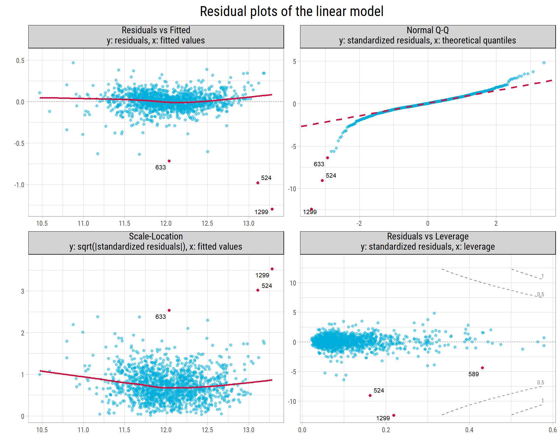
# standardized residual, leverage and Cook's distance of each property
dfLmDiagnostics <- tibble(Id = dfTrain_Proc$Id,
                          std_resid = rstandard(model_lm_check),
                          leverage = hatvalues(model_lm_check),
                          cooks = cooks.distance(model_lm_check)) %>%
  arrange(desc(cooks))
lm_diagnostic <- function(propertyId, column) dfLmDiagnostics[[column]][dfLmDiagnostics$Id == propertyId]- Residuals vs Fitted: Most residuals are close to 0. But three properties have very large negative residuals: the model predicts much higher prices than their actual prices. These are Ids 1299, 524 and 633. In Part 2, we saw that 1299 and 524 are very large properties that sold at low prices.
- Normal Q-Q: The lower tail is much longer than the dashed line. Property 1299 has a standardized residual of -12.4, and property 524 has -9.1. For normally distributed errors, values beyond -3 are very rare.
- Scale-Location: The smooth line goes up at both ends, so the errors are larger for the cheapest and the most expensive properties.
- Residuals vs Leverage: Properties 1299 and 524 have both a large residual and a high leverage (0.22 and 0.16). So they have the largest Cook’s distances, 0.29 and 0.11. These are below the dashed contour at 0.5, but much larger than for most properties. They pull the straight-line fit, which is one reason why
glmnetand the tree-based models work better.
Regularized Linear Model
Next, we use glmnet, a linear model with regularization. Regularization adds a penalty for large coefficients. This makes the model keep only the effects that the data clearly supports. glmnet combines two types of regularization: LASSO (L1), which can reduce the coefficient of a feature to exactly 0, and Ridge (L2), which makes all the coefficients smaller. We search for the values of these hyperparameters that give the lowest RMSE:
penalty: the total amount of regularization in the model.mixture: the share of LASSO (L1) regularization in the model.
model_spec_glmnetLinear Regression Model Specification (regression)
Main Arguments:
penalty = tune()
mixture = tune()
Computational engine: glmnet Here are the 10 best RMSE values and their hyperparameter combinations:
cv_results_glmnet %>% head(10)# A tibble: 10 × 3
penalty mixture mean_rmse
<dbl> <dbl> <dbl>
1 1.46e- 2 0.297 0.129
2 1.22e- 3 0.490 0.130
3 1.09e- 2 0.0439 0.131
4 3.47e- 4 0.992 0.131
5 1.22e- 2 0.657 0.131
6 8.18e- 4 0.0856 0.132
7 7.37e- 7 0.0221 0.132
8 1.15e- 4 0.798 0.132
9 3.37e-10 0.0573 0.133
10 1.57e- 5 0.0760 0.133What’s notable?
- After we choose the hyperparameters with cross validation, the best
glmnetmodel has an RMSE of 0.129, with penalty = 0.0146 and mixture = 0.2974. - This is better than the ordinary least squares model, which had an RMSE of 0.1336. The regularization makes the coefficients of the less useful features smaller. This helps when there are so many features.
- Cross validation of
glmnetis fast. It takes about 13 seconds. - But outliers can strongly affect its results.
Here is a plot of the glmnet hyperparameter grid, with the best combination:
eda_plot_scatter(param_grid_glmnet, "mixture", "penalty", alpha = 1, add_lm = F, yLog = T, yLabelsScale = scales::scientific) +
  geom_point(data = param_best_glmnet, aes(x = mixture, y = penalty), color = "red") +
  ggrepel::geom_label_repel(data = param_best_glmnet %>% map_df(round, digits = 4),
                            aes(x = mixture, y = penalty, label = glue::glue("penalty: {penalty}, mixture:{mixture}")),
                            family = "Roboto Condensed")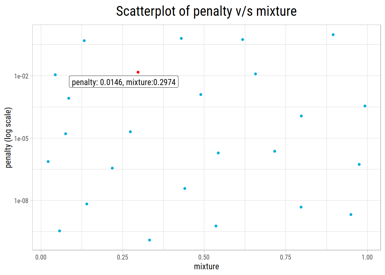
Non-linear Models
Next, we train two types of models that use decision trees. A decision tree predicts a value by asking a series of yes/no questions about the features, such as “Is TotalSF more than 2000?”. These models are not very sensitive to outliers and skewed data.
ranger (Random Forest)
A random forest builds many decision trees, each from a random sample of the data, and takes the average of their predictions. We use ranger, a version of random forests that gives the same results as the randomForest package but runs about 3 times faster. Each forest has 500 trees. (On a dataset of this size, more trees do not improve the error.) We search for the best values of these hyperparameters:
mtry: the number of features that the tree chooses from at random at each question (split).min_n: the minimum number of properties that a group (node) must have before the tree can split it again.
model_spec_rfRandom Forest Model Specification (regression)
Main Arguments:
mtry = tune()
trees = 500
min_n = tune()
Engine-Specific Arguments:
num.threads = 1
Computational engine: ranger Here are the 10 best RMSE values and their hyperparameter combinations:
cv_results_rf %>% head(10)# A tibble: 10 × 3
min_n mtry mean_rmse
<int> <int> <dbl>
1 2 51 0.132
2 12 67 0.134
3 5 81 0.134
4 15 34 0.134
5 9 22 0.135
6 22 42 0.136
7 18 82 0.136
8 8 121 0.137
9 19 108 0.138
10 33 46 0.138What’s notable?
- After cross validation, the best RMSE is 0.132, with mtry = 51 and min_n = 2.
- This is not better than
glmnet. Also, cross validation ofrangertakes much longer: about 279 seconds, against 13 seconds forglmnet.
Here is a plot of the ranger hyperparameter grid, with the best combination:
eda_plot_scatter(param_grid_rf, "min_n", "mtry", alpha = 1, add_lm = F) +
  geom_point(data = param_best_rf, aes(x = min_n, y = mtry), color = "red") +
  ggrepel::geom_label_repel(data = param_best_rf, aes(x = min_n, y = mtry, label = glue::glue("mtry: {mtry}, min_n:{min_n}")), family = "Roboto Condensed")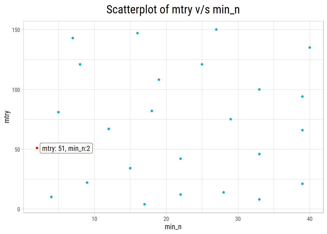
xgboost
xgboost (gradient boosting) builds decision trees one after the other. Each new tree corrects some of the errors of the trees before it. Each model has 1000 trees, and we search for the best values of these hyperparameters:
min_n: the minimum number of properties that a group (node) must have before the tree can split it again.tree_depth: the maximum number of questions (splits) from the top of a tree to its bottom.learn_rate: how much each new tree can change the predictions. A smaller value makes the model learn more slowly and carefully.
model_spec_xgboostBoosted Tree Model Specification (regression)
Main Arguments:
trees = 1000
min_n = tune()
tree_depth = tune()
learn_rate = tune()
Engine-Specific Arguments:
objective = reg:squarederror
nthread = 1
Computational engine: xgboost Here are the 10 best RMSE values and their hyperparameter combinations:
cv_results_xgboost %>% head(10)# A tibble: 10 × 4
min_n tree_depth learn_rate mean_rmse
<int> <int> <dbl> <dbl>
1 33 2 0.0289 0.125
2 3 2 0.0171 0.127
3 23 4 0.0254 0.128
4 24 1 0.190 0.129
5 11 5 0.0549 0.129
6 32 9 0.00605 0.130
7 19 11 0.00482 0.130
8 16 14 0.0121 0.131
9 38 9 0.0270 0.131
10 23 9 0.0405 0.131What’s notable?
- After cross validation, the best RMSE is 0.125, with min_n = 33, tree_depth = 2 and learn_rate = 0.0289.
- This is the best cross validated RMSE of all the models. It is a little better than
glmnet(0.129) andranger(0.132). - Cross validation of
xgboosttakes longer thanglmnet, but it is faster thanranger(about 177 seconds).
Finalizing Models
For each model, we now know the hyperparameters with the lowest RMSE. We use them to train each model again on the complete training set. Then we use the trained models to predict log(SalePrice) for the training set, and we compare the predictions with the actual values.
# Get predicted estimates
get_predicted <- function(model_final, dfNew) {

  # Predict on testing set
  vEstimates <- model_final %>%
    predict(new_data = dfNew) %>%
    pull(.pred)

  return(vEstimates)
}

dfResults_train <- dfTrain %>%
  mutate(actual = log(SalePrice)) %>%
  select(Id, actual) %>%
  mutate(glmnet = get_predicted(model_final = model_final_glmnet, dfTrain_Proc),
         ranger = get_predicted(model_final = model_final_rf, dfTrain_Proc),
         xgboost = get_predicted(model_final = model_final_xgboost, dfTrain_Proc))
dfPlot <- dfResults_train %>%
gather(model, predicted, -actual, -Id) %>%
mutate(model = ordered(model, levels = c("glmnet","ranger","xgboost")))
dfPlot %>%
rename(`log(SalePrice)` = actual) %>%
eda_plot_predicted_vs_actual("log(SalePrice)", "predicted", feature_model = "model", feature_id = "Id", nLabel = 3) +
labs(title = "Predicted v/s actual log(SalePrice) on training set")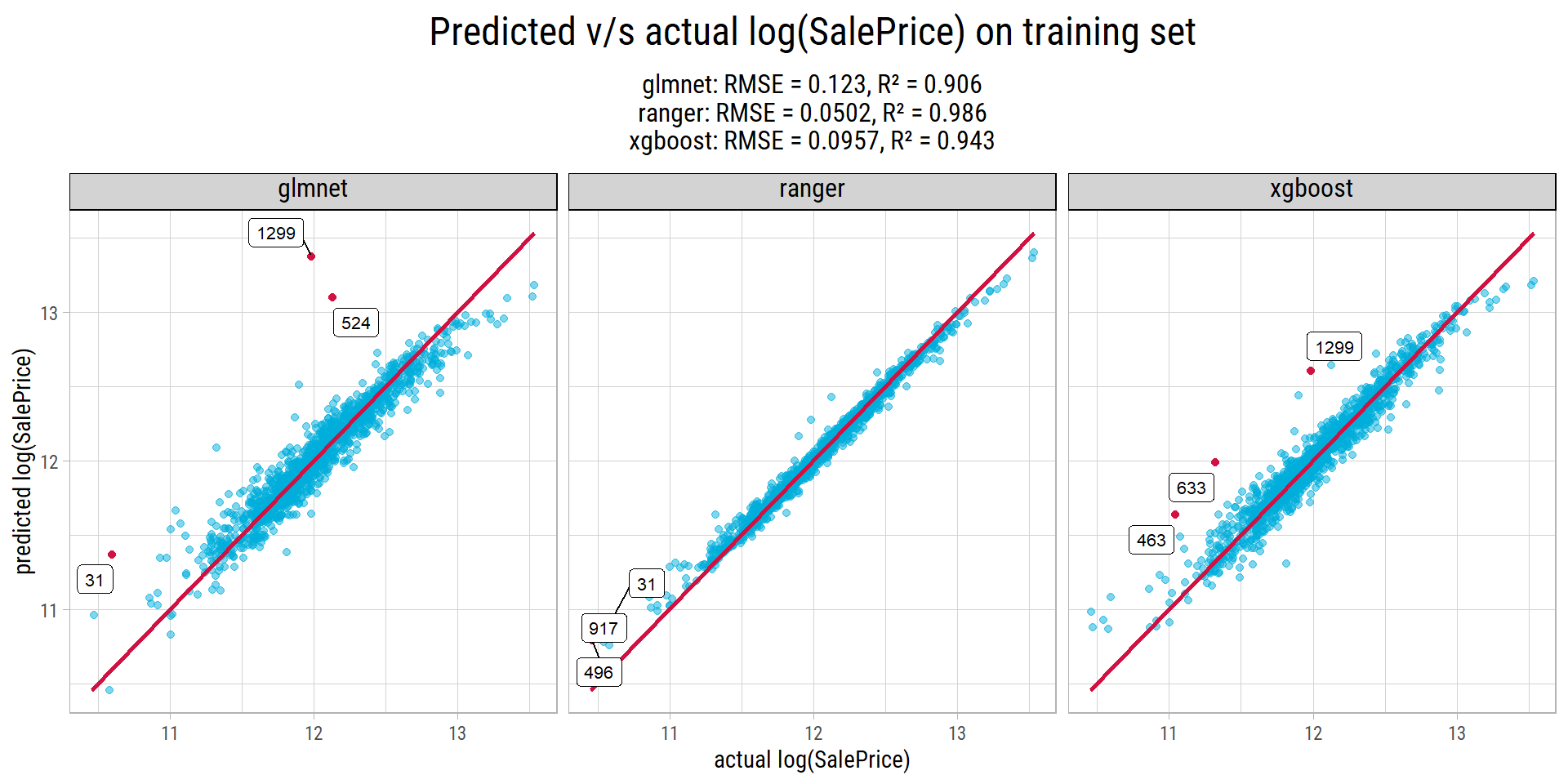
# properties among the 3 largest errors of more than one model
dfWorst_train <- dfPlot %>%
  group_by(model) %>%
  slice_max(abs(predicted - actual), n = 3) %>%
  ungroup() %>%
  count(Id, name = "n_models") %>%
  filter(n_models > 1) %>%
  arrange(desc(n_models))

# sentence about the properties that are among the largest errors of the most models
worst_train_sentence <- if (nrow(dfWorst_train) == 0) {
  "No property is among them for more than one model."
} else {
  vIds <- dfWorst_train$Id[dfWorst_train$n_models == max(dfWorst_train$n_models)]
  glue::glue("{if (length(vIds) == 1) 'The property with Id' else 'The properties with Ids'} {paste0('__', vIds, '__', collapse = ' and ')} {if (length(vIds) == 1) 'is' else 'are each'} among them for {max(dfWorst_train$n_models)} of the 3 models, so we should check {if (length(vIds) == 1) 'its' else 'their'} data for errors.")
}
What’s notable?
rangerandxgboostfit the training data closely: their predictions are near the 45-degree line, where the predicted value is equal to the actual value.rangerfits the training data most closely, with a training RMSE of 0.050, against 0.096 forxgboost.- The
glmnetmodel has two outliers, Ids 524 and 1299. Their predicted prices are much higher than their actual prices, so their points are far above the line. Also, for the cheaper properties, the predicted values are very spread out. - The plots label the three largest errors of each model. The properties with Ids 31 and 1299 are each among them for 2 of the 3 models, so we should check their data for errors.
- But a good fit on the training data does not prove that a model is good. We can only measure its true performance on data that it has not seen: the testing set.
Performance on Test Data
dfResults_test <- dfTest %>%
  mutate(actual = log(SalePrice)) %>%
  select(Id, actual) %>%
  mutate(glmnet = get_predicted(model_final = model_final_glmnet, dfTest_Proc),
         ranger = get_predicted(model_final = model_final_rf, dfTest_Proc),
         xgboost = get_predicted(model_final = model_final_xgboost, dfTest_Proc))
dfPlot <- dfResults_test %>%
gather(model, predicted, -actual, -Id) %>%
mutate(model = ordered(model, levels = c("glmnet","ranger","xgboost")))
dfPlot %>%
rename(`log(SalePrice)` = actual) %>%
eda_plot_predicted_vs_actual("log(SalePrice)", "predicted", feature_model = "model", feature_id = "Id", nLabel = 3) +
labs(title = "Predicted v/s actual log(SalePrice) on testing set")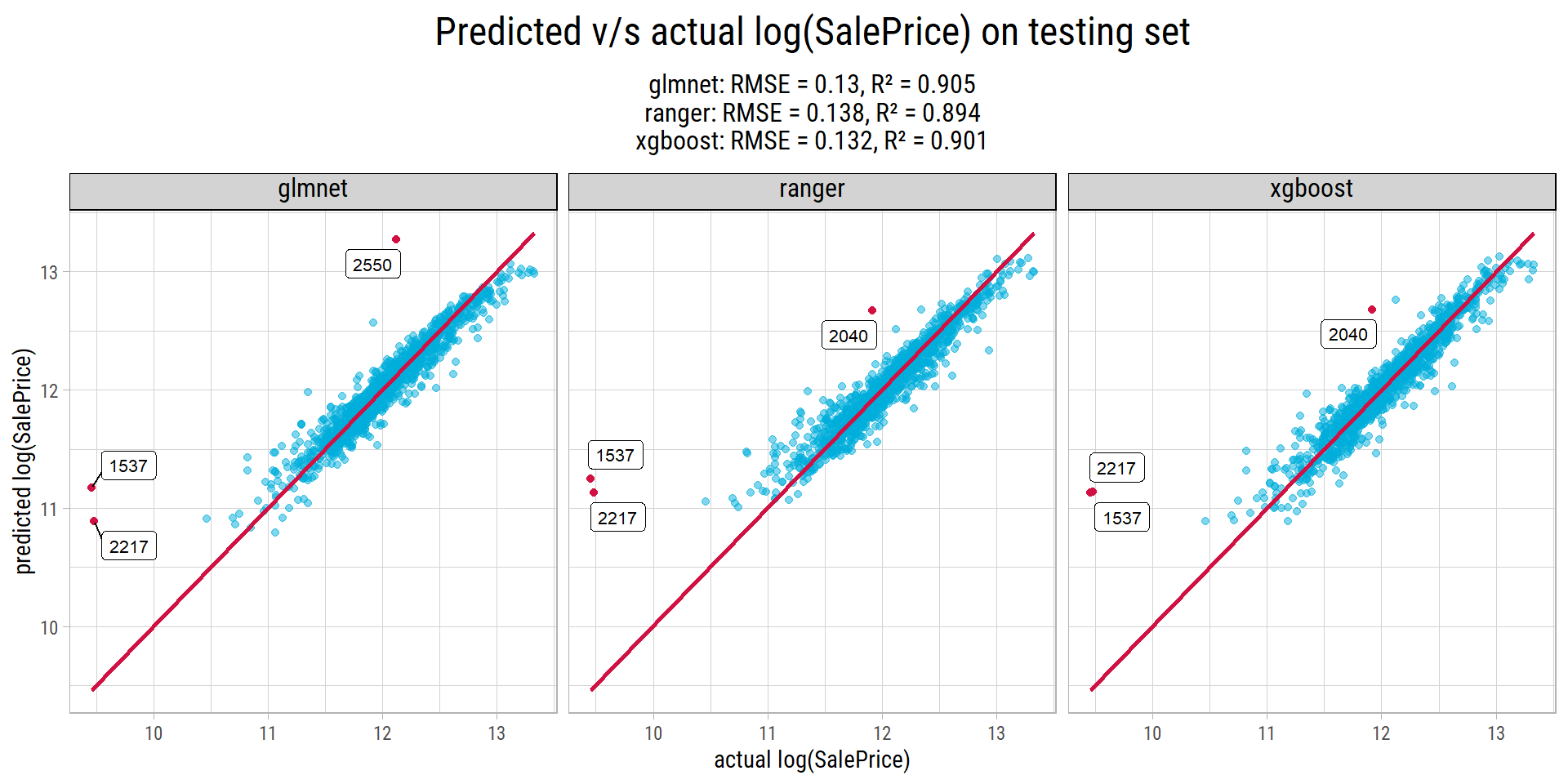
dfRMSE <- map(list("glmnet","ranger","xgboost"), ~ rmse(dfResults_test, actual, !!sym(.x)) %>% mutate(model = .x)) %>%
  bind_rows() %>%
  mutate(cv_rmse = c(cv_results_glmnet$mean_rmse[1], cv_results_rf$mean_rmse[1], cv_results_xgboost$mean_rmse[1])) %>%
  select(-.estimator, -.metric) %>%
  rename(test_rmse = .estimate) %>%
  select(model, everything())

dfRMSE
# A tibble: 3 × 3
model test_rmse cv_rmse
<chr> <dbl> <dbl>
1 glmnet 0.130 0.129
2 ranger 0.138 0.132
3 xgboost 0.132 0.125What’s notable?
- For all the models, the RMSE on the testing set is similar to the cross validated RMSE. This shows that cross validation correctly estimated how well the models work on new data, and that the hyperparameters are good.
- The properties with Ids 1537 and 2217 are outliers: no model predicts a price close to their actual prices.
glmnethas the lowest RMSE on the testing set, 0.130.xgboostis close, with 0.132.- But outliers affect
glmnet, as we saw with Ids 524 and 1299 in the training set.xgboosthad the best cross validated RMSE, and the difference on the testing set is small. Also,xgboostis less affected by outliers, and it can learn curved relationships. So we choosexgboostas our final model, because it works well on new data.
model_final <- model_final_xgboostFeature Importance
It is harder to understand how xgboost makes its predictions than how a linear model makes them. But a variable importance plot can show which features are the most important for the model.
Here are the 10 most important features of our final xgboost model:
library(vip)

p1 <- vip(extract_fit_parsnip(model_final), aesthetics = list(fill = "#00AED8")) +
  labs(title = "xgboost model Feature Importance in Training") +
  theme_quant()

vFeaturesImp <- vip::vi(extract_fit_parsnip(model_final)) %>% top_n(10, Importance) %>% pull(Variable)

p2 <- eda_plot_correlation_matrix(dfTrain %>% select(SalePrice, one_of(vFeaturesImp)),
                            outlineVar = "SalePrice", plotTitle = "Correlations with SalePrice")

cowplot::plot_grid(plotlist = list(p1, p2), nrow = 1)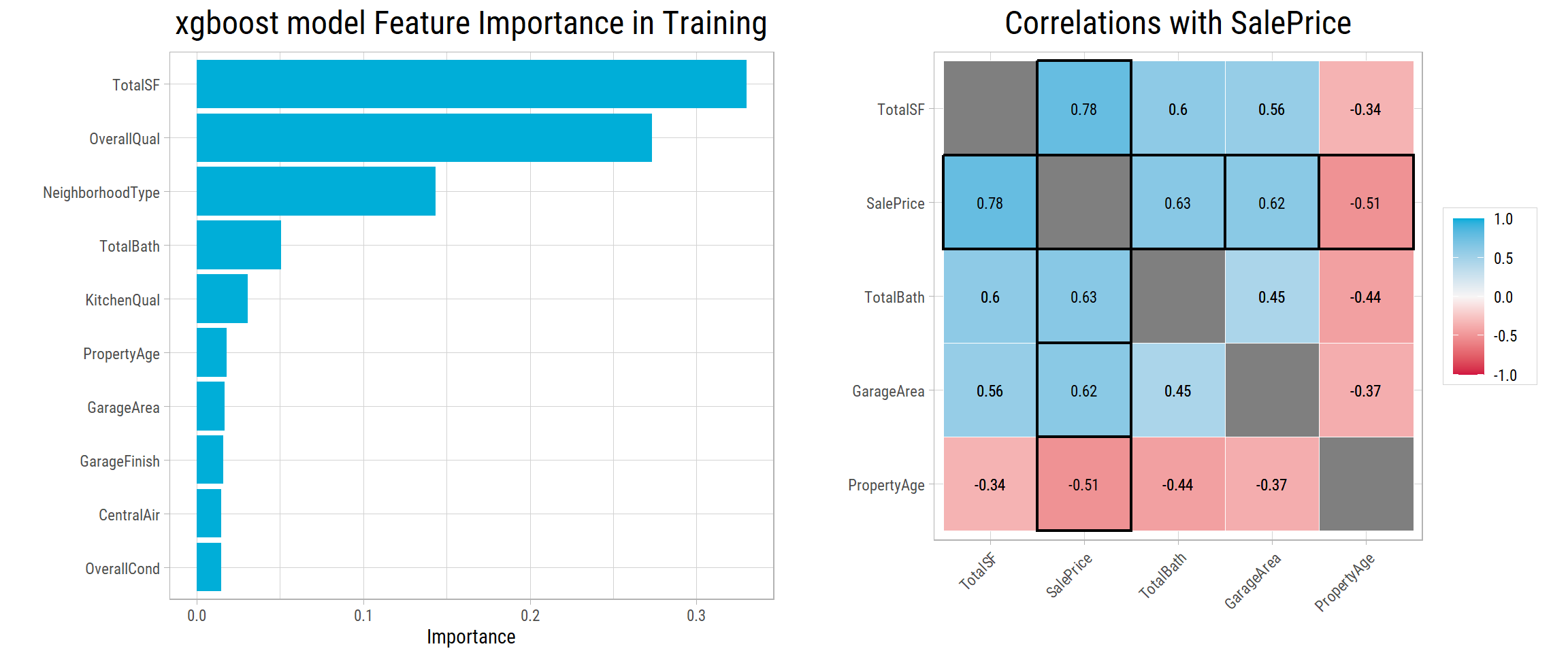
- The plot on the right shows the correlations of the numerical features. All of them have a correlation of at least 0.5, or at most -0.5, with
SalePrice. - All of the 10 most important features make sense. To judge the price of a property, a buyer would look at the total area, the overall quality, the neighborhood, the number of bathrooms, the kitchen quality, the age of the property, the size and finish of the garage, central air conditioning, the overall condition, and so on.
- So our final model works well on new data, and it chooses very reasonable features.
New Property Premium
Of the 10 most important features in our final model, most do not change during the life of a property, such as the area, the neighborhood and the number of bathrooms. The quality and the condition of a property can change, but people judge them in different ways. The only feature that clearly changes over time is PropertyAge.
So, how does the predicted SalePrice change with the age of a property? We compare the same property when it is new, when it is more than 30 years old, and at all the ages in between.
We choose two properties at random, change their PropertyAge, and look at the effect on the predicted SalePrice.
getSampleProperty <- function(randomSeed) {

  set.seed(randomSeed)
  dfSample <- dfTest %>%
    filter(PropertyAge >= 30) %>%
    sample_n(1)

  dfSample <- tibble(PropertyAge = 1:dfSample$PropertyAge[1]) %>% expand_grid(dfSample %>% select(-PropertyAge))
}

dfSample <- getSampleProperty(1000) %>% bind_rows(getSampleProperty(2000))

# preprocess the sample data with the recipe prepared on the training set and generate predicted values from the final model
bake(preprocessing_recipe, new_data = dfSample) %>%
  get_predicted(model_final, .) %>%
  as_tibble() %>%
  bind_cols(dfSample) %>%
  mutate(predicted = exp(value)) %>%
  group_by(Id) %>%
  ggplot(aes(x = PropertyAge, y = predicted)) +
  geom_point(color = "#00AED8") +
  geom_line() +
  facet_wrap(~Id, scales = "free") +
  scale_y_continuous(labels = scales::label_dollar(accuracy = 1)) +
  labs(y = "Predicted Sale Price",
       title = "New Property Premium")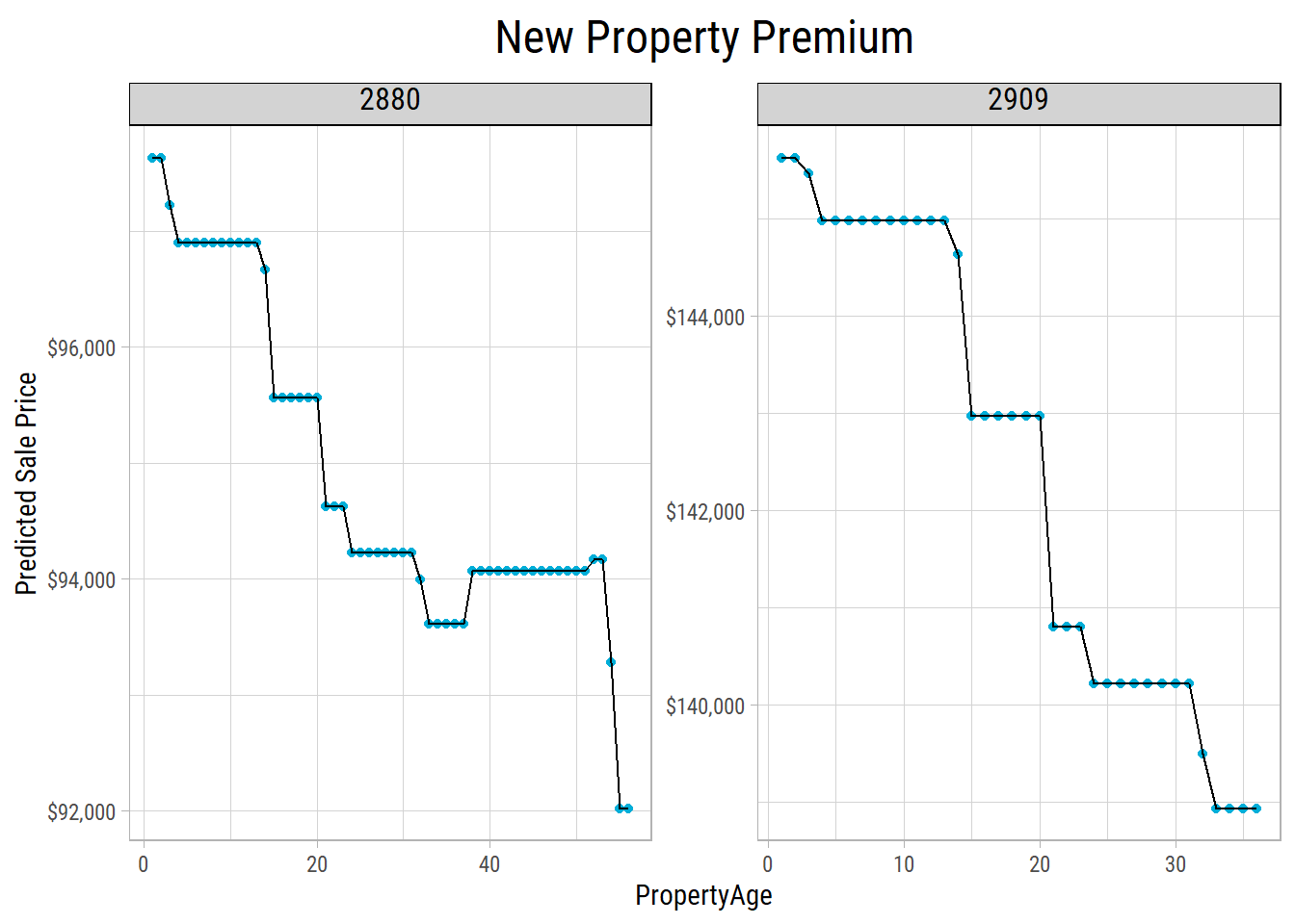
A new property sells for a little more than an older property of the same type, quality and condition. This premium is small in a place like Ames, Iowa. We expect it to be much higher in a large city.
Appendix: Tuning Code
This is the code that tunes the models. It takes several minutes, so it does not run each time we build this page. Instead, the page saves the results in the file Ames_Tuning.Rda, together with a fingerprint (a hash) of the inputs of the tuning. The inputs are the clean data from Part 1 and the tuning code itself, which also sets the hyperparameter grids. When we build the page again, it calculates the fingerprint again:
- If the fingerprint is the same, the page loads the saved results in a few seconds.
- If the data, a hyperparameter or any other part of the tuning code has changed, the page tunes the models again and saves the new results.
Changes to the comments or the spacing of the code do not count as changes. To tune the models again without any change, delete Ames_Tuning.Rda.
These are the tuning steps:
# Why the tuning code is built the way it is (speed):
# The dataset is small (1,460 rows x ~150 predictors after encoding), so run time is driven by the
# number of model fits (5 models x 25 grid points x 5 folds) and by how expensive each fit is, not by data size.
# The earlier version took ~35 minutes; this version takes ~11 minutes with 6 workers, tuning the same models and
# hyperparameters (with randomForest replaced by the equivalent ranger engine). The changes:
#   1. tune_grid() parallelises over every fold x grid-point combination ("everything"), instead of a manual
#      for-loop over grid points that only ran the 5 folds in parallel and left the remaining cores idle.
#   2. Random forest uses only the `ranger` engine with 500 trees. The `randomForest` package was tuned in addition
#      to ranger and gave the same cross-validated RMSE (0.135 vs 0.134). On one fold with mtry = 84, min_n = 2:
#        randomForest, 1,000 trees: 46.9s, RMSE 0.1305
#        ranger,       1,000 trees: 15.1s, RMSE 0.1303
#        ranger,         500 trees:  7.2s, RMSE 0.1293
#      Random forest error levels off well before 500 trees on data of this size, so 1,000 trees only doubled the cost.
#   3. xgboost searches a sensible learning-rate range, instead of spending much of the grid on learning rates as
#      small as 1e-10 that cannot converge in 1,000 rounds (see get_model_param_grid). Early stopping was tried and
#      rejected; see the note in get_model_spec.
#   4. The number of parallel workers is capped by available RAM as well as CPU cores (see "Parallel backend").
#
# Unrelated to speed: the earlier version used Id as a predictor. It is now excluded (see get_workflow).
# It also had 21 predictors that were exact linear combinations of others, which lm reported as a rank-deficient
# fit. They are now removed (see "Collinear predictors" and get_preprocessing_recipe), leaving a full-rank design.
# Ordered factors are encoded as integer scores instead of polynomial contrasts (see get_preprocessing_recipe).

# load the clean dataset from Part 1 (ames_data_file is set in the "tuning_cache" chunk)
load(ames_data_file)

# Collinear predictors
########################################################################################################################################################
# With the earlier set of features, 21 of the ~250 predictors were exact linear combinations of others (the design
# matrix had rank 229 of 250), so lm could not estimate them and warned of a rank-deficient fit. Tree models are not
# affected by duplicated information, but linear models are: the coefficients of collinear predictors are unstable.
# These features are dropped because other features already carry their information (see the association matrix
# in Part 1):
#   HasGarage, HasFireplace, HasMasVnr: the same as the "None" category of GarageType, FireplaceQu and MasVnrType.
#   MSSubClass: combines the building type and style, already in BldgType and HouseStyle (bias-corrected Cramer's V
#               of 0.89 and 0.83). Its "duplex" category is identical to BldgType's.
#   HalfBath:   TotalBath = FullBath + 0.5 * HalfBath + BsmtBath exactly. Dropping HalfBath rather than TotalBath
#               keeps the total, one of the most important features for the tree models, and loses no information
#               because HalfBath can be recovered from the other three.
vFeaturesCollinear <- c("HasGarage", "HasFireplace", "HasMasVnr", "MSSubClass", "HalfBath")

# Categories that no property has (e.g. a Poor exterior quality) are dropped too, so that the scores of ordered factors
# are consecutive (see get_preprocessing_recipe).
dfClean <- dfClean %>%
    select(-all_of(vFeaturesCollinear)) %>%
    mutate(across(where(is.factor), droplevels))

# Determine skewed features
vFeaturesSkew <- dfClean %>%
    select_if(is.numeric) %>%
    select_if(function(Z) abs(timeDate::skewness(Z, na.rm = T)) > 0.75) %>%
    colnames() %>%
    setdiff(c("Id","PropertyAge"))

# Remove Outliers and split clean data
########################################################################################################################################################
# dfClean <- dfClean %>% dplyr::filter(!(Id %in% c(524, 1299))) # glmnet cv_rmse improves to 0.117 but test_rmse is 0.135
dfTrain <- dfClean %>% filter(!(Id %in% vTestIDs))
dfTest <- dfClean %>% filter(Id %in% vTestIDs)

# Preprocessing Recipe
########################################################################################################################################################
# Ordered factors (quality and condition grades, etc.) are encoded as integer scores, one predictor per feature, in
# the order of their categories. The alternative, step_dummy's polynomial contrasts, creates one predictor per category
# but one. Grades that only a handful of properties have can then be missing from a cross validation fold, which makes
# the highest-order contrasts collinear: with that encoding lm reported a rank-deficient fit in 4 of the 5 folds. Scores
# assume the grades are equally spaced, which is a reasonable approximation for these grades, and they cut the
# number of predictors from ~214 to ~151. dfEncodingComparison below compares the two encodings.
#
# step_lincomb removes any remaining exact linear combinations among the predictors. These can arise because properties
# without a basement or garage share the "None" category of every basement or garage feature. An intercept column is
# added for the check, because such combinations can include a constant, and removed afterwards.
get_preprocessing_recipe <- function(df, ordinalScores = TRUE) {

    preprocessing_recipe <- recipe(SalePrice ~ ., data = df) %>%
        update_role(Id, new_role = "ID") %>%
        step_mutate_at(one_of(vFeaturesSkew), -all_outcomes(), fn = ~ log(. + 1L))
    if(ordinalScores) {
        preprocessing_recipe <- preprocessing_recipe %>%
            step_ordinalscore(all_ordered_predictors())
    }
    preprocessing_recipe <- preprocessing_recipe %>%
        step_dummy(all_nominal()) %>%
        step_intercept() %>%
        step_lincomb(all_numeric_predictors()) %>%
        step_rm(any_of("intercept")) %>%
        step_log(all_outcomes()) %>%
        prep()
    return(preprocessing_recipe)
}

# The recipe is prepared on the training set only, and the same recipe is applied to the testing set (and to any new
# data), so that both have exactly the same predictors.
preprocessing_recipe <- get_preprocessing_recipe(dfTrain)

# Preprocessed data for training models
dfTrain_Proc <- preprocessing_recipe %>%
    bake(new_data = NULL) %>%
    rename(target = SalePrice) %>%
    select(target, everything())

dfTest_Proc <- preprocessing_recipe %>%
    bake(new_data = dfTest) %>%
    rename(target = SalePrice) %>%
    select(target, everything())


# Create cv folds
########################################################################################################################################################
get_cv_folds <- function(df, numFolds, strataVar, randomSeed, shuffleData) {
    # shuffle the rows
    if(shuffleData) {
        set.seed(randomSeed)
        df <- df[sample(nrow(df)), ]
    }

    # split dataset into folds where each fold has the same distribution of target
    lFolds <- df %>% vfold_cv(v = numFolds, strata = all_of(strataVar))
    return(lFolds)
}


# Parsnip Model Specification
########################################################################################################################################################
get_model_spec <- function(modelType) {

    model_spec <- switch(modelType,
                         lm = linear_reg(mode = "regression") %>%
                             set_engine("lm"),

                         glmnet = linear_reg(mode = "regression", penalty = tune(), mixture = tune()) %>%
                             set_engine("glmnet"),

                         # No early stopping. It was tried (stop after 50 rounds without improvement on a 10% validation split)
                         # and roughly halved xgboost tuning time, but the final model was unstable: refitting the same best
                         # parameters with different random validation splits stopped anywhere from 195 to 687 rounds, with test
                         # RMSE between 0.133 and 0.151, versus 0.131 for a fixed 1,000 trees. With only ~146 validation rows the
                         # stopping point is too noisy. The narrower learn_rate range already removes the wasted fits.
                         # nthread = 1 because parallelism comes from running many fits at once (one per worker).
                         xgboost = boost_tree(mode="regression", trees=1000, min_n=tune(), tree_depth=tune(), learn_rate=tune()) %>%
                             set_engine("xgboost", objective = "reg:squarederror", nthread = 1),

                         kernlab = svm_rbf(mode="regression", cost=tune(), rbf_sigma=tune(), margin=tune()) %>%
                             set_engine("kernlab"),

                         # ranger replaces the randomForest engine: same algorithm, ~3x faster implementation, and 500 trees
                         # instead of 1,000 with no loss of accuracy (see the timings at the top of this code).
                         # num.threads = 1 for the same reason as xgboost's nthread above.
                         ranger = rand_forest(mode = "regression", trees = 500, mtry = tune(), min_n = tune()) %>%
                             set_engine("ranger", num.threads = 1))

    return(model_spec)
}


# Parameter Grid Search
########################################################################################################################################################
get_model_param_grid <- function(df, modelType, numParams, randomSeed) {

    # mtry is finalized on the predictors only, so its upper bound is the number of predictors (excludes target and Id)
    dfPredictors <- df %>% select(-target, -Id)

    set.seed(randomSeed)
    param_spec <- switch(modelType,
                         glmnet = parameters(penalty(), mixture()),
                         kernlab = parameters(cost(), rbf_sigma(), svm_margin()),
                         # learn_rate is on a log10 scale. The dials default (1e-10 to 1e-1) spends most of the grid on rates
                         # so small that 1,000 trees barely move from the starting prediction: those fits take the full time
                         # and are never competitive. 10^-2.5 to 10^-0.5 (~0.003 to ~0.3) covers the useful range; the best
                         # rate found with the default range was ~0.07, comfortably inside it.
                         xgboost = parameters(min_n(), tree_depth(), learn_rate(range = c(-2.5, -0.5))),
                         ranger = parameters(min_n(), finalize(mtry(), dfPredictors)))

    dfParamGrid <- grid_space_filling(param_spec, size = numParams, type = "max_entropy")
    return(dfParamGrid)
}


# Workflow for a model
########################################################################################################################################################
# The data is already preprocessed, so the workflow only names the outcome and predictors.
# Id is excluded from the predictors: it is a row identifier, and with training Ids 1-1460 and test Ids 1461-2919,
# tree models would otherwise split on it and treat every test property as lying beyond the training range.
get_workflow <- function(model_spec) {
    workflow() %>%
        add_variables(outcomes = target, predictors = -Id) %>%
        add_model(model_spec)
}


# Cross Validation Results
########################################################################################################################################################
# tune_grid() fits every grid point on every fold. With parallel_over = "everything", each (fold, grid point)
# combination is a separate task, so all workers stay busy until the end of the run.
# The mean RMSE across folds is the same metric as before (mean of the per-fold RMSE).
cross_validate_model <- function(cv_folds, model_spec, param_grid) {

    tune_results <- get_workflow(model_spec) %>%
        tune_grid(resamples = cv_folds,
                  grid = param_grid,
                  metrics = metric_set(rmse),
                  control = control_grid(parallel_over = "everything"))

    dfResults <- tune_results %>%
        collect_metrics() %>%
        select(all_of(names(param_grid)), mean_rmse = mean) %>%
        arrange(mean_rmse)
    return(dfResults)
}


# Fitted model with parameters
########################################################################################################################################################
# Returns a fitted workflow; predict() on it selects the predictor columns from new data, so Id can stay in the data.
# The seed makes the final ranger and xgboost fits reproducible between runs.
get_fitted_model <- function(df, model_spec, dfParams, randomSeed = 2300) {

    model_wf <- get_workflow(model_spec)
    if(!is.null(dfParams)) model_wf <- model_wf %>% finalize_workflow(dfParams)
    set.seed(randomSeed)
    fit(model_wf, data = df)
}


# Parallel backend
########################################################################################################################################################
# Each worker is a separate R session with tidymodels and the model packages loaded. In a full run with 5 workers,
# no R process exceeded 0.6 GB and all R processes together (main session + workers) peaked at 3.2 GB. Budgeting
# 0.75 GB per worker leaves headroom. Workers are capped at cores - 1 (to keep the machine responsive) and at what fits in 70% of the RAM
# available when the run starts, so the run cannot push the machine into swapping even if other applications are open.
gb_per_worker <- 0.75
gb_available <- ps::ps_system_memory()$avail / 1024^3
num_workers <- max(1, min(parallel::detectCores() - 1, floor(0.7 * gb_available / gb_per_worker)))
message(sprintf("Using %d parallel workers (%.1f GB RAM available)", num_workers, gb_available))
plan(multisession, workers = num_workers)

# Create cross validation folds
cv_folds <- get_cv_folds(dfTrain_Proc, numFolds = 5, strataVar = "target", randomSeed = 2300, shuffleData = T)

# Compare the encodings of ordered factors with a linear model on the same folds (reported in the post)
compare_encoding <- function(ordinalScores) {

    df <- get_preprocessing_recipe(dfTrain, ordinalScores) %>%
        bake(new_data = NULL) %>%
        rename(target = SalePrice) %>%
        select(target, everything())
    folds <- get_cv_folds(df, numFolds = 5, strataVar = "target", randomSeed = 2300, shuffleData = T)
    vAliased <- map_int(folds$splits, ~ sum(is.na(coef(lm(target ~ ., data = analysis(.x) %>% select(-Id))))))

    tibble(encoding = if(ordinalScores) "ordinal scores" else "polynomial contrasts",
           predictors = ncol(df) - 2,
           folds_rank_deficient = sum(vAliased > 0),
           lm_cv_rmse = suppressWarnings(get_workflow(get_model_spec("lm")) %>%
                                             fit_resamples(resamples = folds, metrics = metric_set(rmse)) %>%
                                             collect_metrics() %>%
                                             pull(mean)))
}
dfEncodingComparison <- bind_rows(compare_encoding(ordinalScores = FALSE), compare_encoding(ordinalScores = TRUE))

# Time each model so the post can report relative run times
dfTimings <- tibble(model = character(), seconds = numeric())
time_model <- function(model, expr) {
    t0 <- Sys.time()
    result <- force(expr)
    dfTimings <<- dfTimings %>% add_row(model = model, seconds = as.numeric(difftime(Sys.time(), t0, units = "secs")))
    result
}

# lm model (no hyperparameters, so fit_resamples instead of tune_grid)
model_spec_lm <- get_model_spec(modelType = "lm")
cv_results_lm <- time_model("lm",
    get_workflow(model_spec_lm) %>%
        fit_resamples(resamples = cv_folds, metrics = metric_set(rmse)) %>%
        collect_metrics() %>%
        select(mean_rmse = mean))

# glmnet model
model_spec_glmnet <- get_model_spec(modelType = "glmnet")
param_grid_glmnet <- get_model_param_grid(dfTrain_Proc, modelType = "glmnet", numParams = 25, randomSeed = 2300)
cv_results_glmnet <- time_model("glmnet", cross_validate_model(cv_folds, model_spec_glmnet, param_grid_glmnet))
param_best_glmnet <- cv_results_glmnet %>% slice(1) %>% select(-mean_rmse)
model_final_glmnet <- get_fitted_model(dfTrain_Proc, model_spec_glmnet, param_best_glmnet)

# kernlab model
model_spec_kernlab <- get_model_spec(modelType = "kernlab")
param_grid_kernlab <- get_model_param_grid(dfTrain_Proc, modelType = "kernlab", numParams = 25, randomSeed = 2300)
cv_results_kernlab <- time_model("kernlab", cross_validate_model(cv_folds, model_spec_kernlab, param_grid_kernlab))
param_best_kernlab <- cv_results_kernlab %>% slice(1) %>% select(-mean_rmse)
model_final_kernlab <- get_fitted_model(dfTrain_Proc, model_spec_kernlab, param_best_kernlab)

# random forest model (ranger engine; objects keep the _rf names used in index.Rmd)
model_spec_rf <- get_model_spec(modelType = "ranger")
param_grid_rf <- get_model_param_grid(dfTrain_Proc, modelType = "ranger", numParams = 25, randomSeed = 2300)
cv_results_rf <- time_model("ranger", cross_validate_model(cv_folds, model_spec_rf, param_grid_rf))
param_best_rf <- cv_results_rf %>% slice(1) %>% select(-mean_rmse)
model_final_rf <- get_fitted_model(dfTrain_Proc, model_spec_rf, param_best_rf)

# xgboost model
model_spec_xgboost <- get_model_spec(modelType = "xgboost")
param_grid_xgboost <- get_model_param_grid(dfTrain_Proc, modelType = "xgboost", numParams = 25, randomSeed = 2300)
cv_results_xgboost <- time_model("xgboost", cross_validate_model(cv_folds, model_spec_xgboost, param_grid_xgboost))
param_best_xgboost <- cv_results_xgboost %>% slice(1) %>% select(-mean_rmse)
model_final_xgboost <- get_fitted_model(dfTrain_Proc, model_spec_xgboost, param_best_xgboost)

plan(sequential)

# the results that the post uses, which are saved to Ames_Tuning.Rda
vTuningResults <- c("model_spec_lm", "model_spec_glmnet", "model_spec_rf", "model_spec_xgboost", "model_spec_kernlab",
                    "model_final_glmnet", "model_final_rf", "model_final_xgboost", "model_final_kernlab", "cv_results_lm",
                    "cv_results_glmnet", "cv_results_rf", "cv_results_xgboost", "cv_results_kernlab", "param_grid_glmnet",
                    "param_grid_rf", "param_grid_xgboost", "param_grid_kernlab", "param_best_glmnet", "param_best_rf",
                    "param_best_xgboost", "param_best_kernlab", "dfTrain", "dfTest", "dfTrain_Proc",
                    "dfTest_Proc", "dfTimings", "get_preprocessing_recipe", "preprocessing_recipe", "vFeaturesCollinear",
                    "dfEncodingComparison", "cv_folds", "vFeaturesSkew")
And this code decides whether to load the saved results or to run the tuning steps:
# The clean dataset from Part 1
ames_data_file <- "../ames-housing-part1-data-pipeline/Ames_Housing_Clean.Rda"

# Fingerprint (hash) of the inputs of the tuning: the data that it uses, and the code of the "tuning_steps"
# chunk, which also sets the hyperparameter grids. Comments and spacing are removed from the code first, so
# editing them does not start a new tuning run.
envData <- new.env()
load(ames_data_file, envir = envData)
tuning_steps <- knitr::knit_code$get("tuning_steps")
tuning_hash <- rlang::hash(list(data = list(envData$dfClean, envData$vTestIDs),
                                code = deparse(parse(text = tuning_steps, keep.source = FALSE))))

# If the saved results were made from the same inputs, load them. Otherwise, tune the models again and save
# the new results together with the fingerprint of their inputs.
envSaved <- new.env()
if (file.exists("Ames_Tuning.Rda")) load("Ames_Tuning.Rda", envir = envSaved)
if (identical(envSaved$tuning_hash, tuning_hash)) {
  list2env(as.list(envSaved), envir = environment())
} else {
  eval(parse(text = tuning_steps))
  save(list = c(vTuningResults, "tuning_hash"), file = "Ames_Tuning.Rda")
}
rm(envData, envSaved)