How Much Do Swimmers Improve in a Season?
In my previous post, we’ve seen how kids improve year-by-year in swimming. Certainly kids get stronger and faster as they grow. But how much impact does practice and coaching have? As I mentioned in my previous post, coaches do not keep a record of attendance during practice. There are daily hour long practice sessions during the summers. But even though it isn’t known how regular the kids are in attending practice, the number of meets that a kid participates in during the season, can be a good proxy. Afterall, it’s highly unlikely that a kid participates in meets while mostly skipping practice.
To judge improvement in a stroke, we’d like to see whether a kid got enough opportunities to practice as well as participate in meets. The summer league lasts for about 2 months. So, a reasonable start would be to take the data of kids whose first and last meet participations in a stroke were spaced at least 4 weeks apart.
Let’s see the distribution of the number of meets those kids participate in a season:
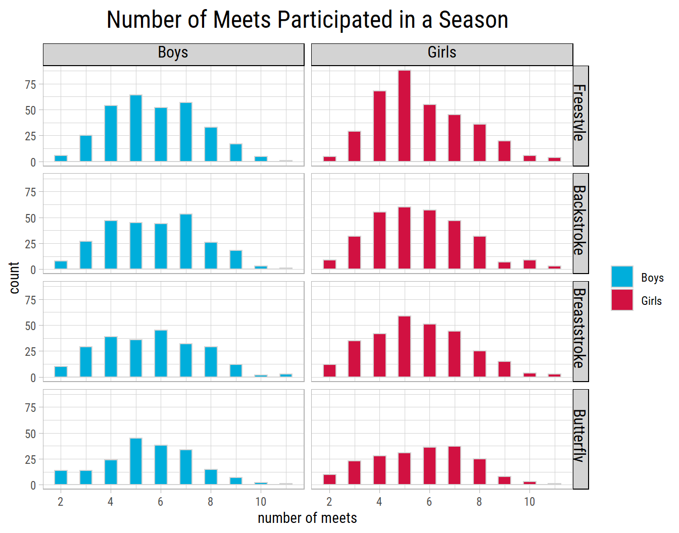
Seems like, for every stroke, most kids participate in 4 or more meets in a season. So we’ll select it as a threshold to judge improvement. Then, for each kid who participates in 4 or more meets in a season, the improvement will be the difference between the first and the last swim times of the season.
Estimating Improvement
Here are the distributions of improvement in swim times by age:
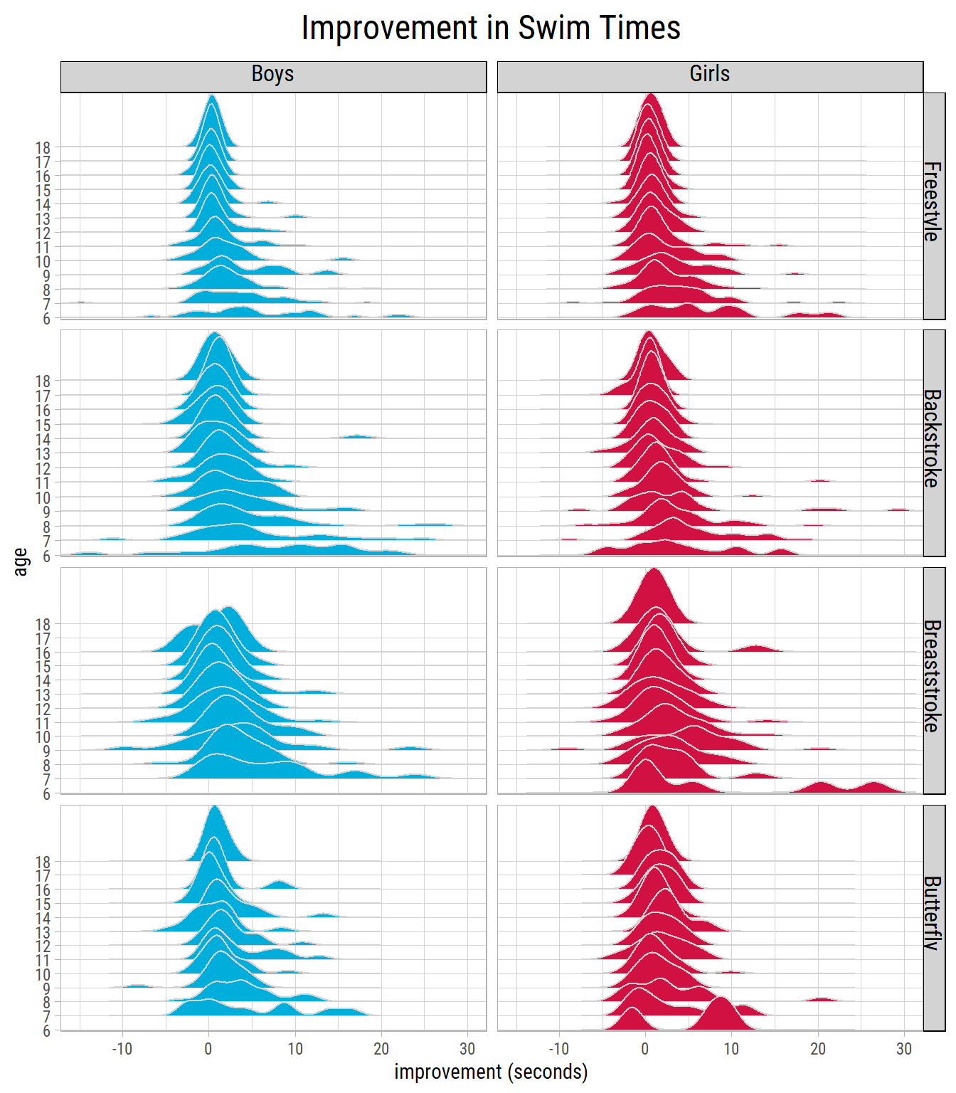
We see wide variance among 6 to 10 year olds. But as the kids grow older, the variance reduces.
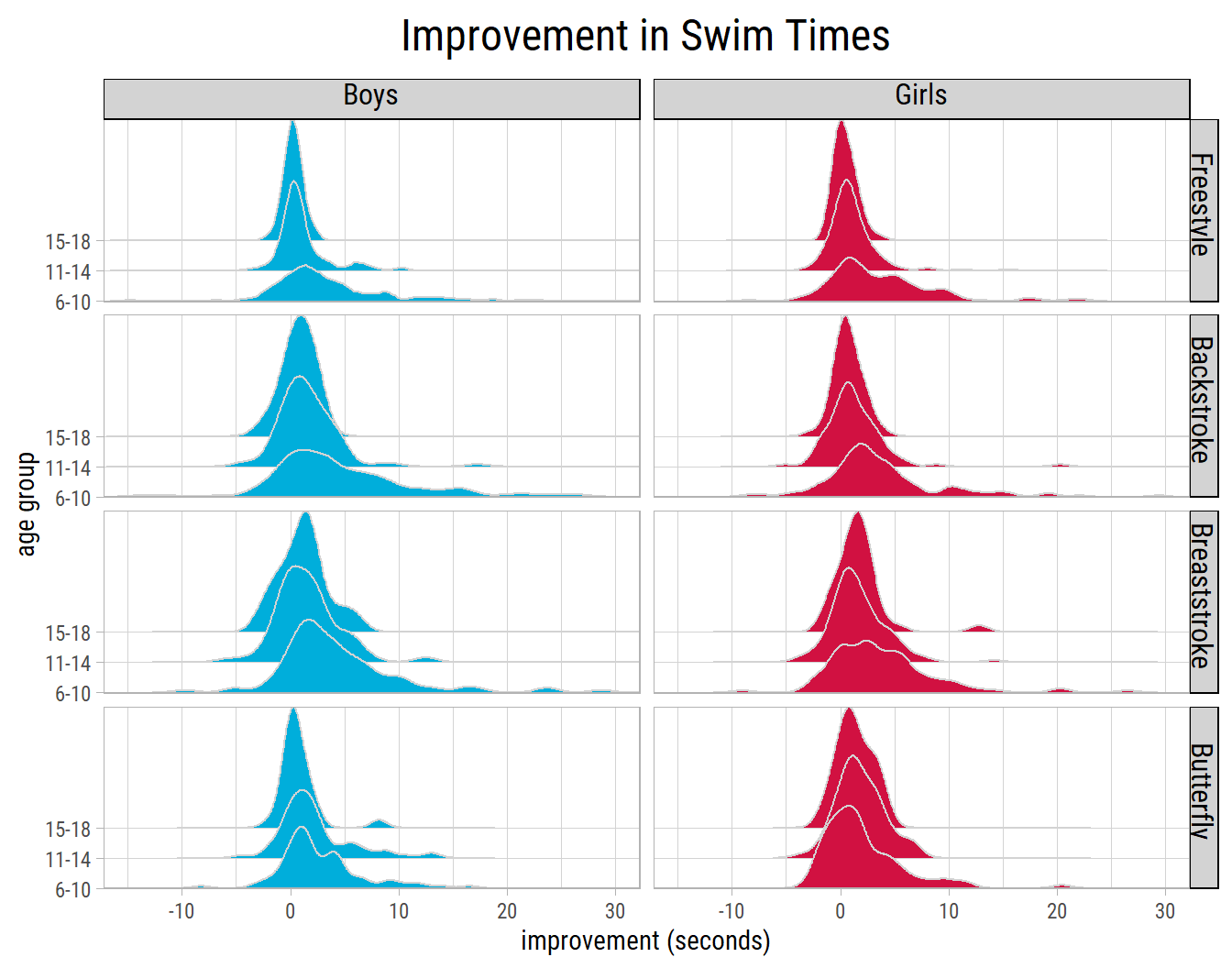
In Breaststroke and Butterfly, there aren’t any 6 year old boys who satisfy the criteria for inclusion. So, instead of looking at improvement by age, it would be better to categorize it by age groups. We could classify kids into 3 age groups, younger kids (6-10), pre-teens and early teens (11-14) and mid to late teens (15-18).
Let’s see a similar plot by age groups:
Is Improvement Significant?
Now that we know the distribution of improvement in swim times, the question arises, is it statistically significant? In other words, does practice and coaching have a significant effect within a short season? It is hard to tell from the plot of distributions itself. Within each age group and stroke, we have a paired sample of swim times, where for the same swimmer, we know their first and last swim times of a season. By using statistical tests, we could quantify mean improvements and determine whether or not they are significant.
Frequentist Method
In traditional statistics, a statistical test known as dependent-samples t test can be used to evaluate whether there is a significant difference between the means of first and last swim times of a season. The null hypothesis is that any change in mean swim times is due to random chance.
Let’s run this test on the sample of Freestyle swim times of 15-18 year old boys.
    Paired t-test

data:  first_time_of_season and last_time_of_season
t = 1.8, df = 31, p-value = 0.08
alternative hypothesis: true difference in means is not equal to 0
95 percent confidence interval:
 -0.03343  0.52031
sample estimates:
mean of the differences
                 0.2434
The mean improvement is about 0.24 seconds, but the 95% confidence interval includes 0, which means we cannot reject the null hypothesis.
Let’s look at the mean improvement and 95% confidence intervals for all the age groups, plotted below:
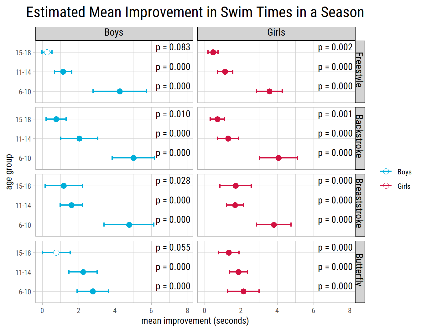
Looking at the plot, we could say girls of all age groups show a statistically significant improvement in swim times in all the strokes. But for boys, the picture is not so clear cut. Boys aged 6-10 and 11-14 show all around statistically significant improvement. But, as seen before, in Freestyle and also in Butterfly, boys aged 15-18 do not. In both the latter cases, confidence intervals include zero. Point estimates are shown with a hollow circle.
But look closely at the p values. Even though the improvements in Backstroke and Breaststroke among 15-18 year old boys appear to be statistically significant, it is only because of the arbitrary choice of 95% confidence level, which has become a de facto standard in published research. With p values of 0.01 and 0.028, we wouldn’t reject the null hypothesis under a 99% confidence level.
If this were a study to be published by a researcher in an academic journal, there would be a temptation to run multiple experiments with different filter criteria and attempt to produce final results according to their own bias; a.k.a. p-hacking.
Under the null hypothesis, we’d draw the conclusion that 15-18 year old boys do not show any statistically significant improvement in a season. We might interpret that the hard work they put in practice is barely enough to maintain their time during a season. With a biased view, we might even question whether they’re putting in as much hard work as the girls of their age.
But, would either of these conclusions be correct? Afterall, girls of all age groups and most boys show statistically significant improvement. So, why would 15-18 year old boys be any different?
Bayesian Method
This is where a Bayesian approach works best. Instead of determining whether the mean difference between the first and last swim times of the season is zero, which is uninformative, the Bayesian way is to determine how much have mean swim times improved, with associated probabilities.
Let’s see the results from a Bayesian counterpart to the t test, on a sample of Freestyle swim times of 15-18 year old boys.
    Bayesian estimation supersedes the t test (BEST) - paired samples

data: first_time_of_season and last_time_of_season, n = 32

  Estimates [95% credible interval]
mean paired difference: 0.24 [-0.026, 0.50]
sd of the paired differences: 0.70 [0.45, 0.96]

The mean difference is more than 0 by a probability of 0.96
and less than 0 by a probability of 0.04
Instead of p-values, this Bayesian test provides an actual probability of improvement in swim times. We get estimates for mean and standard deviation of swim time improvements, along with credible or high density intervals. The probability that the mean improvement is more than zero is 95.9%, though the estimate is less precise and the 95% confidence interval includes zero.
Let’s run the Bayesian test for all strokes and age groups in both genders:
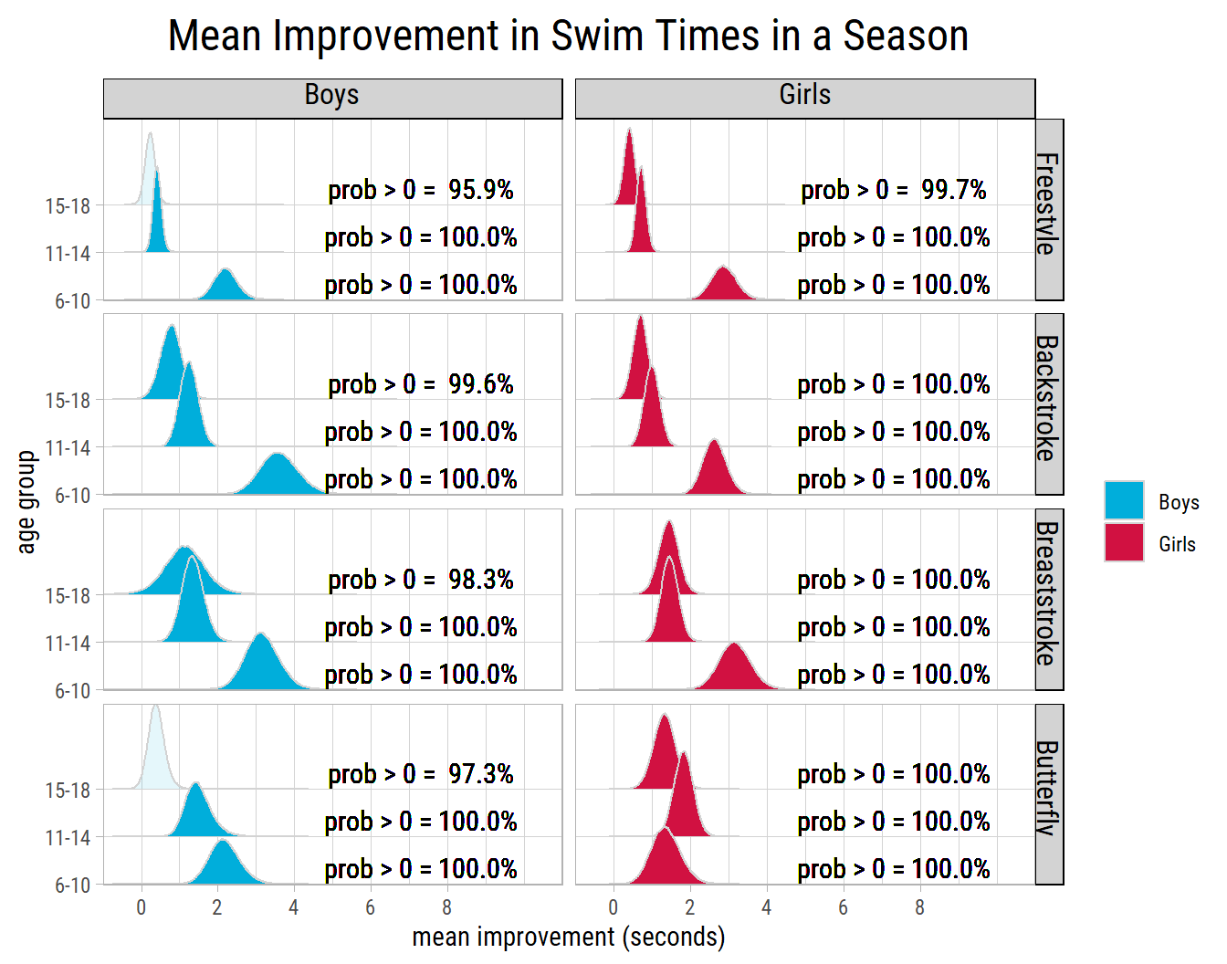
Looking at the distributions, we can see that 15-18 year old boys show a very small improvement in their Freestyle and Butterfly times, but the estimate is less precise and the confidence intervals include zero (those distributions are shaded with a light blue color). Nevertheless the probability of mean improvement being greater than zero is in the high 90s, which from a practical standpoint, is convincing enough.
Conclusion
With a reasonable set of filters, we created sample datasets by age groups to determine whether kids show significant improvement in swim times within a short summer season. We applied Bayesian testing which turns out to be more informative than traditional statistical testing. For all intents and purposes, we can conclude that kids of all age groups show improvement in their swim times, even within a short summer season.
The R markdown file with code for this post is available here.